Examples
All examples follow the package import policy: bring each module in under a stable alias and qualify every call. Only a minimal set of names is exported at the top level — the sweep entry points (coarse_grain, coarse_grain!, coarse_grain_profile, coarse_grain_batch!, coarse_grain_slices!), their result types, check_setup, the three headline kernels, and plot_Π_map/plot_spectrum. Everything else — filter_field!, compute_Π!, compute_Π_strain_convergence, compute_Π_decomposed, tau_decomposition, tracer_variance_flux, enstrophy_flux, band_energies, the remaining kernels, backends, mask strategies, Spectral()/RealSpace() — is reached through its submodule (CGEF.Filtering..., CGEF.Diagnostics..., CGEF.Kernels..., CGEF.ComputationalBackends...), never a flattened top-level re-export. Geometries and grid types come from FlowGeometries.jl.
using CoarseGrainingEnergyFluxes: CoarseGrainingEnergyFluxes as CGEF
using FlowGeometries: FlowGeometries as FG
Start here: check_setup
Before running anything, ask what will actually happen. check_setup reports the engine, the backend, what the kernel can and cannot support, and how wide the contaminated band along a coast is — without building a plan, so it is safe even on a configuration whose plan would be enormous.
julia> CGEF.check_setup(grid, CGEF.TopHatKernel(), 6_000.0)
CoarseGrainingEnergyFluxes setup check
  grid            : StructuredGrid{CartesianGeometry,2} (48, 48)   min spacing (1000.0, 1000.0)
  scale ℓ         : 6000.0  = (6.0, 6.0) cells per axis
  kernel          : TopHatKernel
  masking         : ZeroFill
  method          : default for this grid
  backend         : AutoBackend -> SerialBackend
  real-space engine: prefix-sum top-hat, exact, O(N·w_y)
  ℓ resolvable    : yes
  supports Π      : yes
  spectrum ≥ 0    : NO
  supports Spectral(): NO
  boundary buffer : (3, 3) cells (contaminated)
  notes:
    1. points within (3, 3) cells of a coast or domain edge are contaminated by footprint
       truncation, under either mask strategy — exclude them before averaging.
    2. TopHatKernel's |Ĝ|² is not monotone, so a spectral density is not guaranteed
       non-negative: `coarse_grain` needs `kernel = GaussianKernel()`, or
       `spectrum = Diagnostics.ForceSpectrum()` to compute it anyway, or
       `spectrum = Diagnostics.NoSpectrum()` to skip it.
    3. TopHatKernel's spectral transfer function is provided by a weak dependency that is not
       loaded, so `method = Spectral()` is unavailable in this session — run
       `using SpecialFunctions`. Real-space filtering is unaffected.
Every field is readable programmatically too (r.supports_spectrum, r.boundary_buffer_cells, …), so a script can gate on it rather than parse the text.
Result shapes and conventions
What every result field's axes mean. Ns = length(scales); the spatial rank R is whatever the grid claims, and any array axis beyond that is a batch axis.
| entry point | field | shape | notes |
|---|---|---|---|
coarse_grain/coarse_grain! | Π | (spatial…, Ns) | one contiguous array, not a vector of maps; Π[…, i] is scales[i] |
scales, wavenumber | (Ns,) | wavenumber = L/ℓ | |
cumulative_energy, filtering_spectrum | (Ns,) | filtering_spectrum is NaN under NoSpectrum() | |
coarse_grain_batch! | Π | (spatial…, Ns, batch…) | batch axes trailing, so each slice is a contiguous view |
cumulative_energy, filtering_spectrum, wavenumber | (Ns, batch…) | ||
slices[t] | CoarseGrainResult | a zero-copy view into the batched storage | |
coarse_grain_profile | Π | (Nx, Ny, Ns, Nlevels) | the vertical is just a batch axis; per-level energies are not summed |
coarse_grain_slices! | results[t] | CoarseGrainResult | ragged: one per slice, shapes differ, so no shared storage |
compute_Π! | Π | (spatial…) or (spatial…, batch…) | the grid's rank fixes the split |
compute_Π_strain_convergence | total, strain, convergence, divergence, strain_magnitude | (spatial…) | total = strain − convergence |
compute_Π_decomposed | total, rotational, cross, divergent | (spatial…) | total is the sum of the other three |
tau_decomposition | L, C, R, each (; xx, xy, yy), or (; xx, xy, xz, yy, yz, zz) given w | (spatial…) | L + C + R = τ exactly |
band_energies | bands | (Ns,) | domain means; with maps = true, band_maps[n] is the pointwise map |
enstrophy_flux | Z | (spatial…) | same gauge as Π |
Two conventions worth stating outright, because getting either wrong changes the numbers:
ℓis a diameter, not a radius. The top-hat spans the disk of radiusℓ/2.- Masked cells are zero in every output, never
NaNand never left uninitialized. Points within theboundary_buffer_cellsreported above are computed but contaminated.
Visual Results
The coarse-graining pipeline
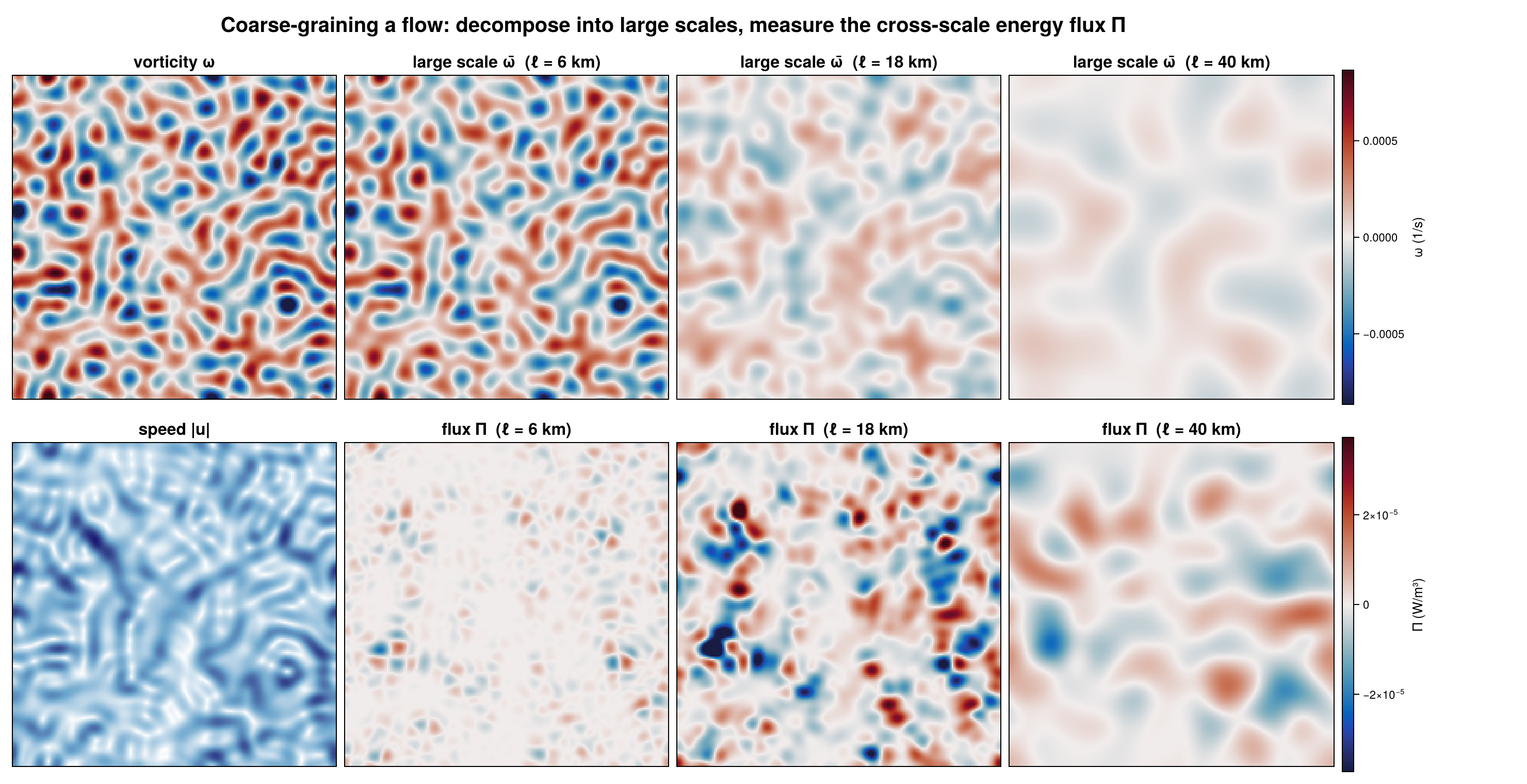
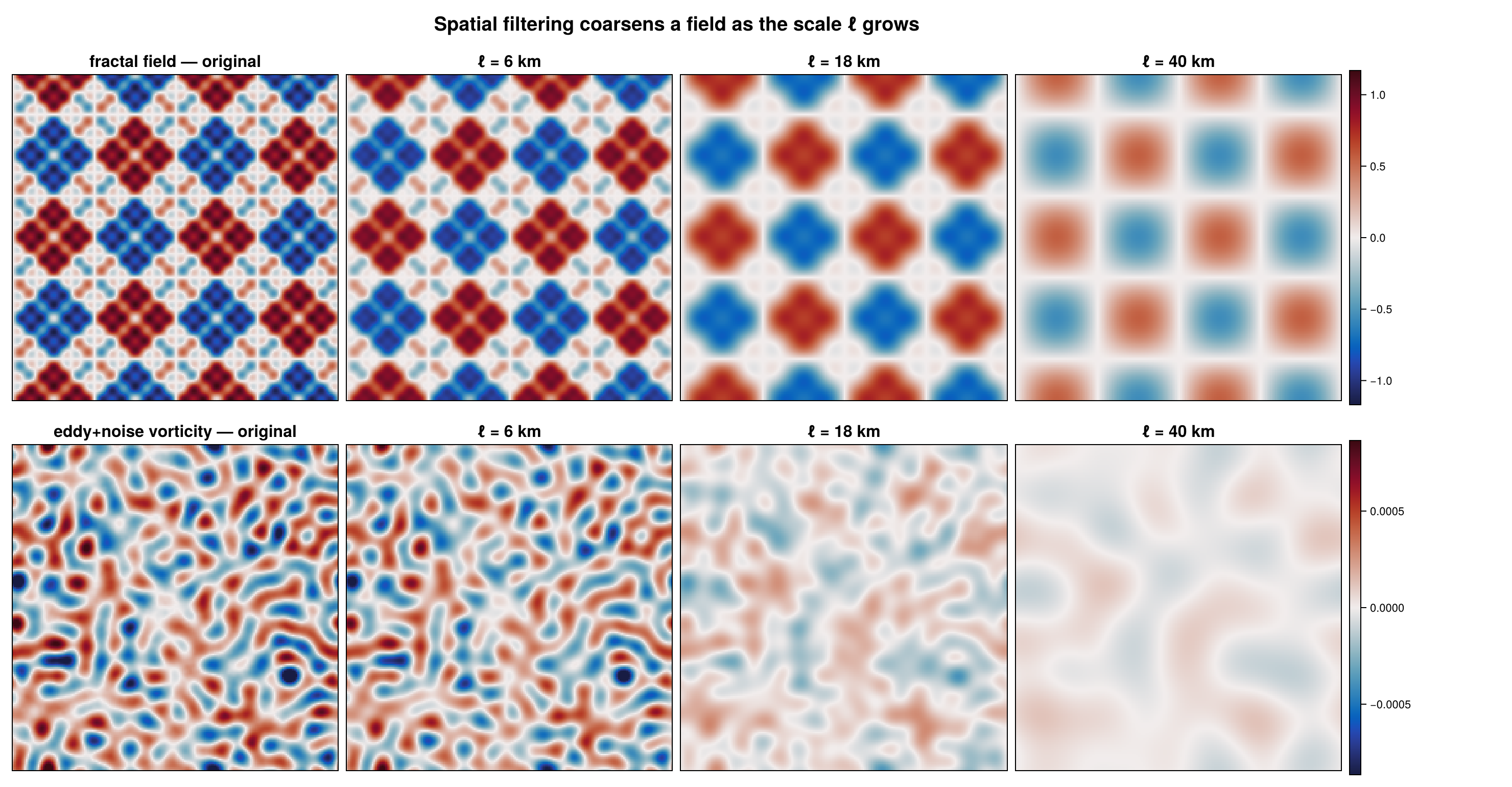
Spatial filtering across scales
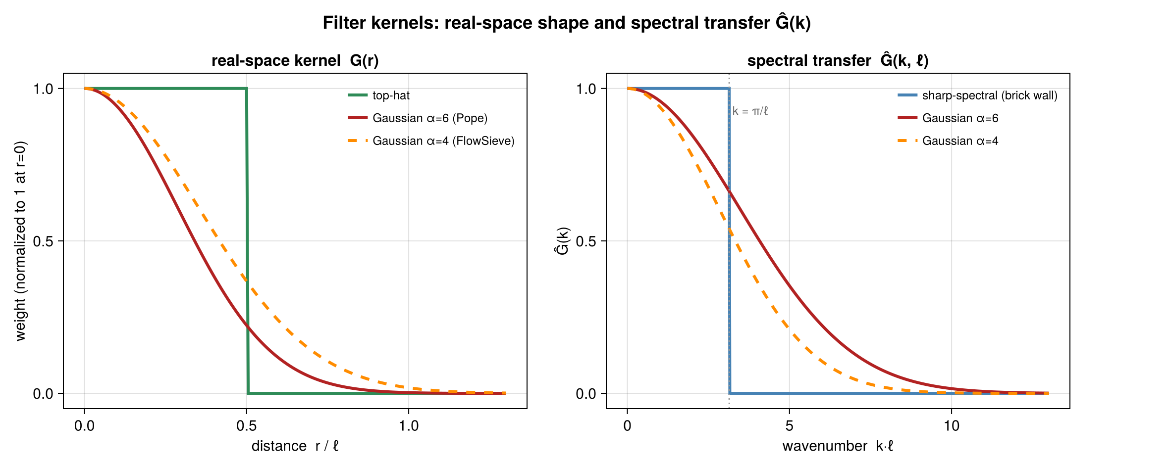
Filter kernels and spectral transfer
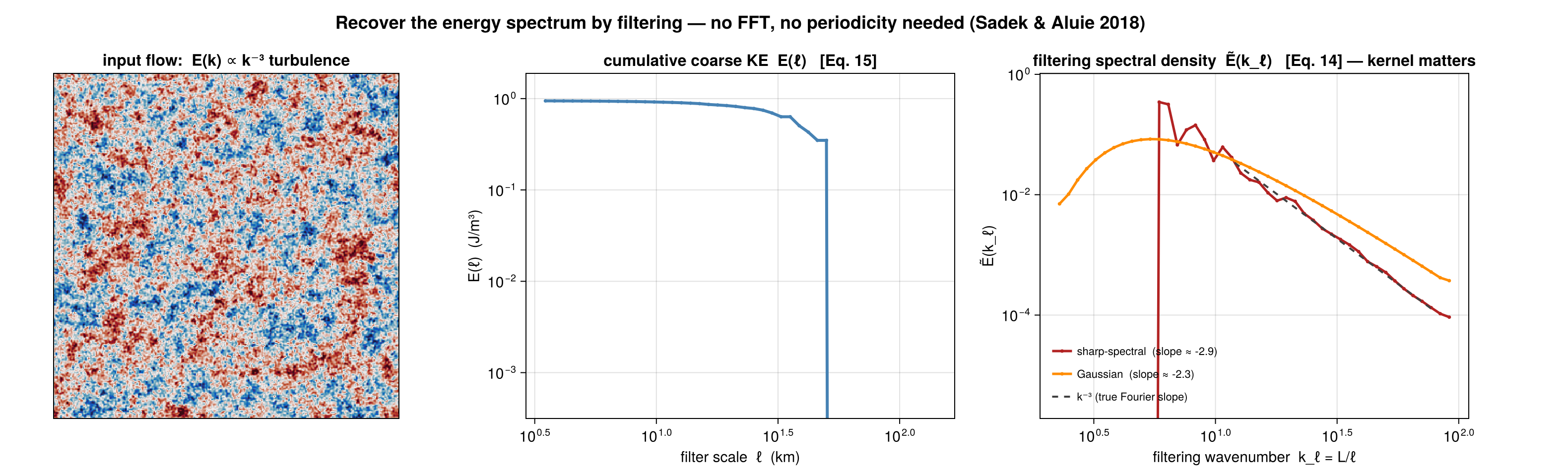
The filtering spectrum (recovers the Fourier slope)
Rotational / divergent (Helmholtz) decomposition of Π
Strain / convergence split of Π
Enstrophy flux (the 2-D companion to Π)
Energy by scale band
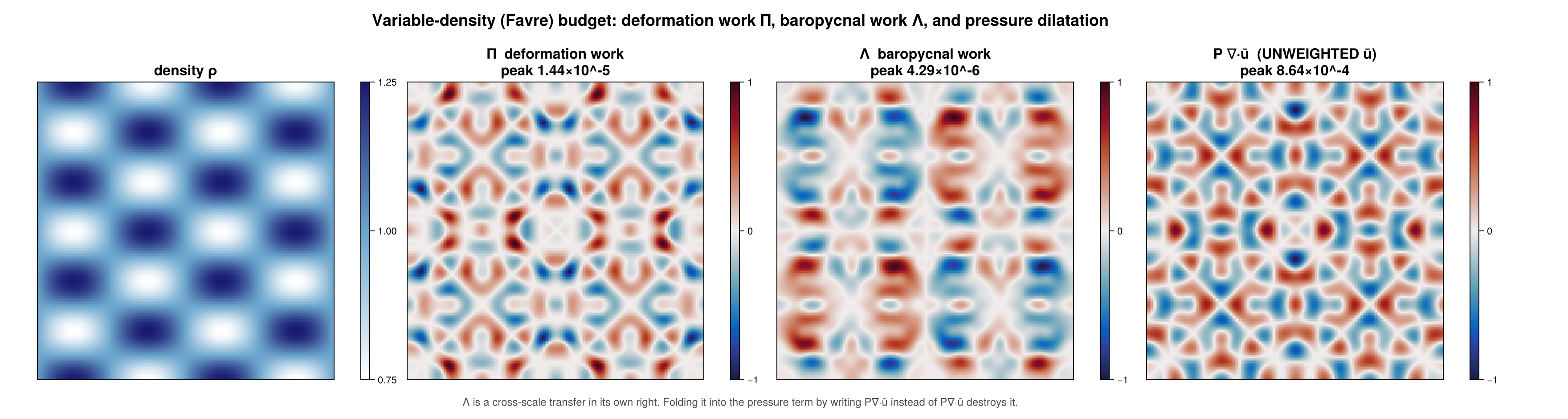
Variable-density (Favre) budget: Π, baropycnal work Λ
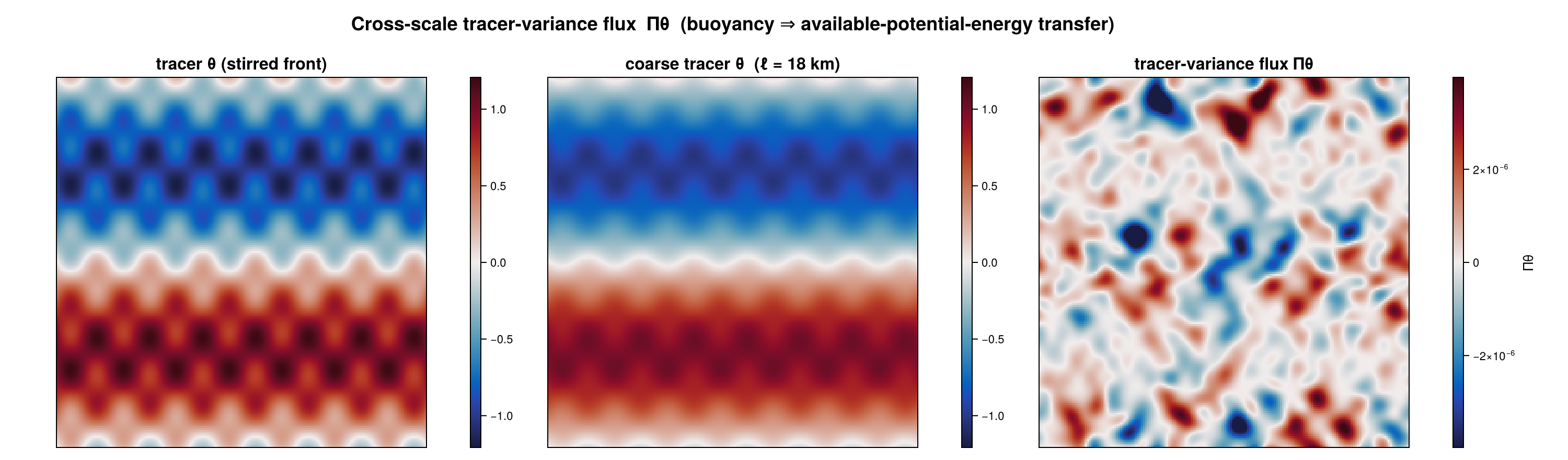
Cross-scale tracer / buoyancy-variance flux
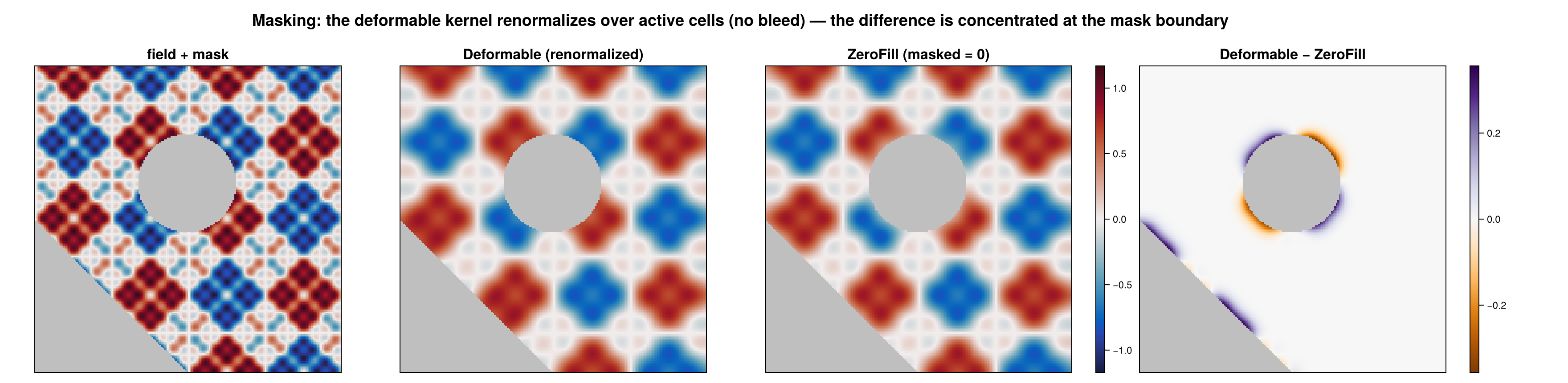
Masking: zero-fill vs deformable
ZeroFill is the default: masked cells contribute nothing and the kernel stays position-independent, so filtering commutes with spatial derivatives — the step the flux budget is derived by. Deformable renormalizes over the locally-active area, reproducing constants exactly next to a boundary at the cost of that commutation. On a masked domain Deformable conserves better (measured 4.8e-4 vs 1.1e-2 relative imbalance); under either choice, points within ≈ℓ of the mask are contaminated.
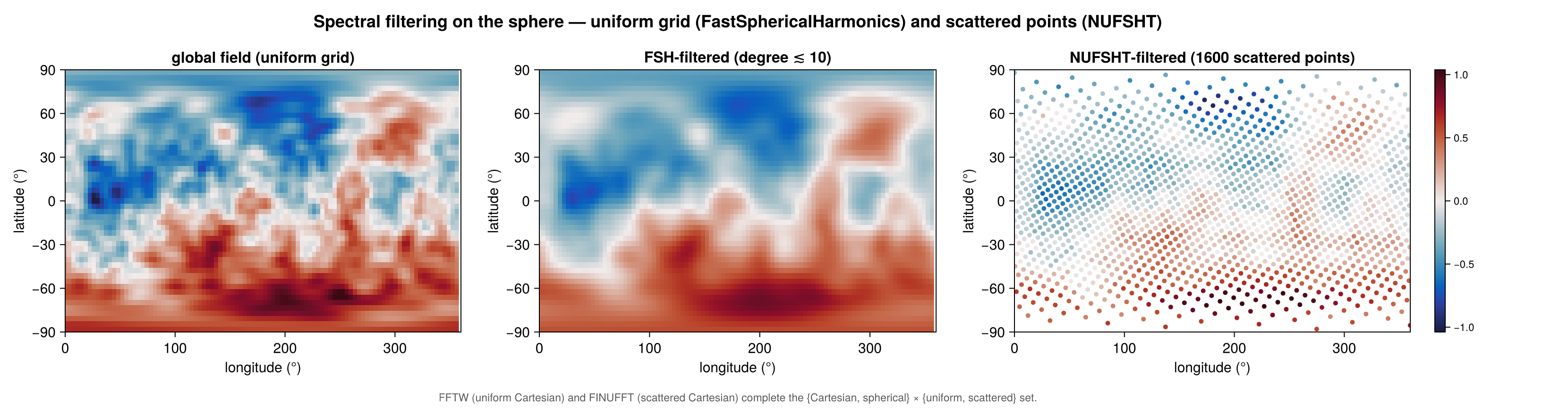
Spectral filtering on the sphere
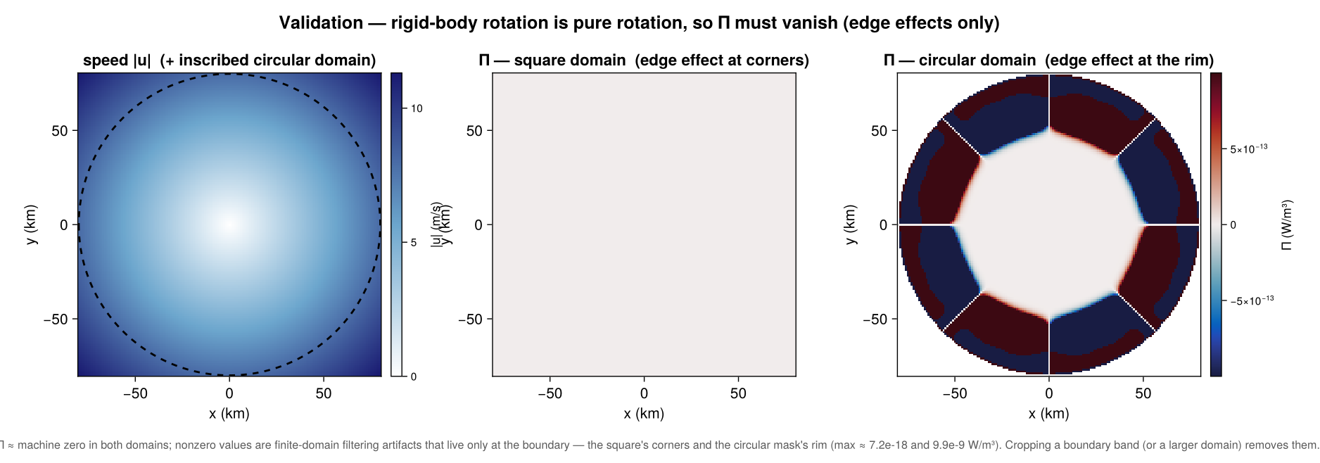
Validation: rigid-body rotation → Π = 0
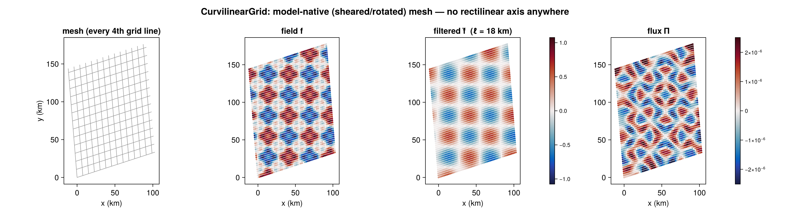
Curvilinear (model-native) grids
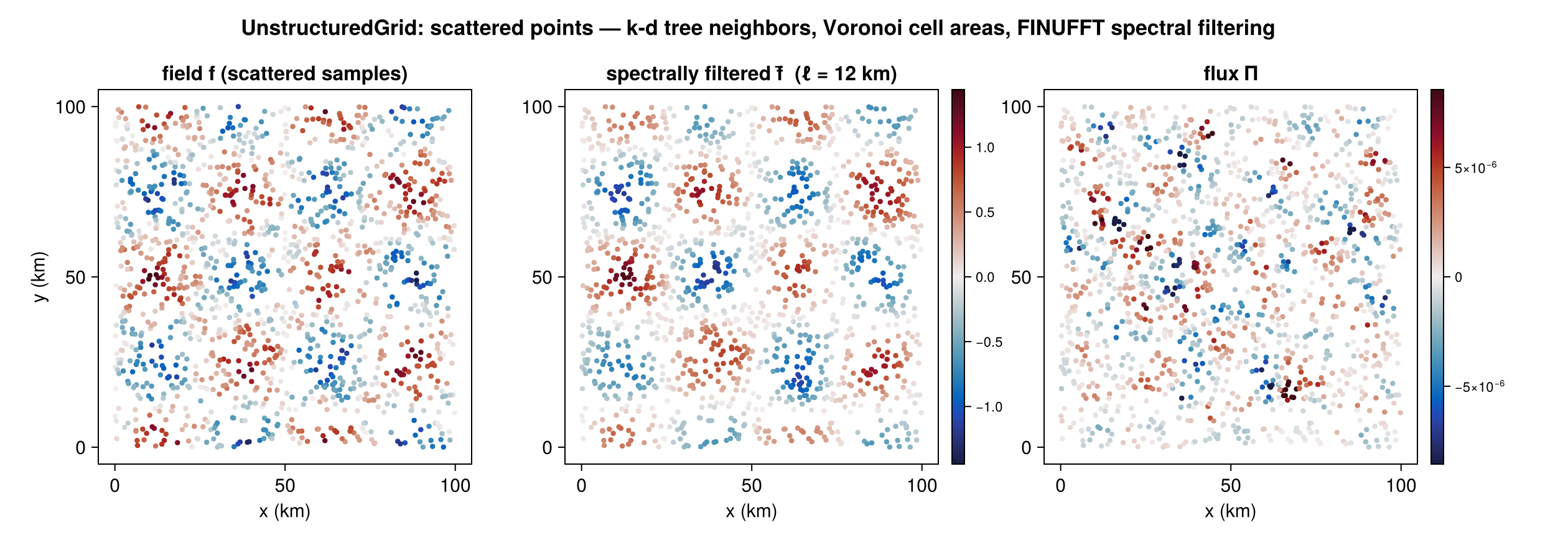
Scattered / unstructured point clouds
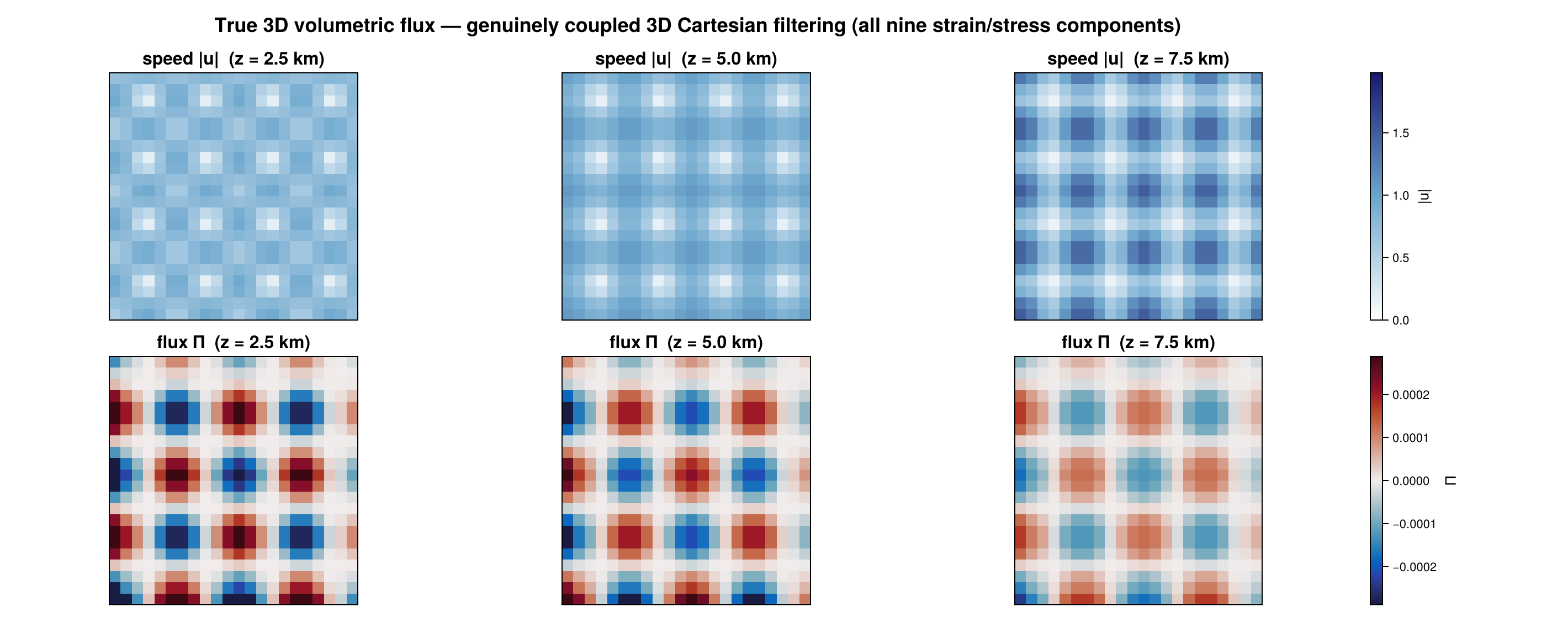
True 3D volumetric flux
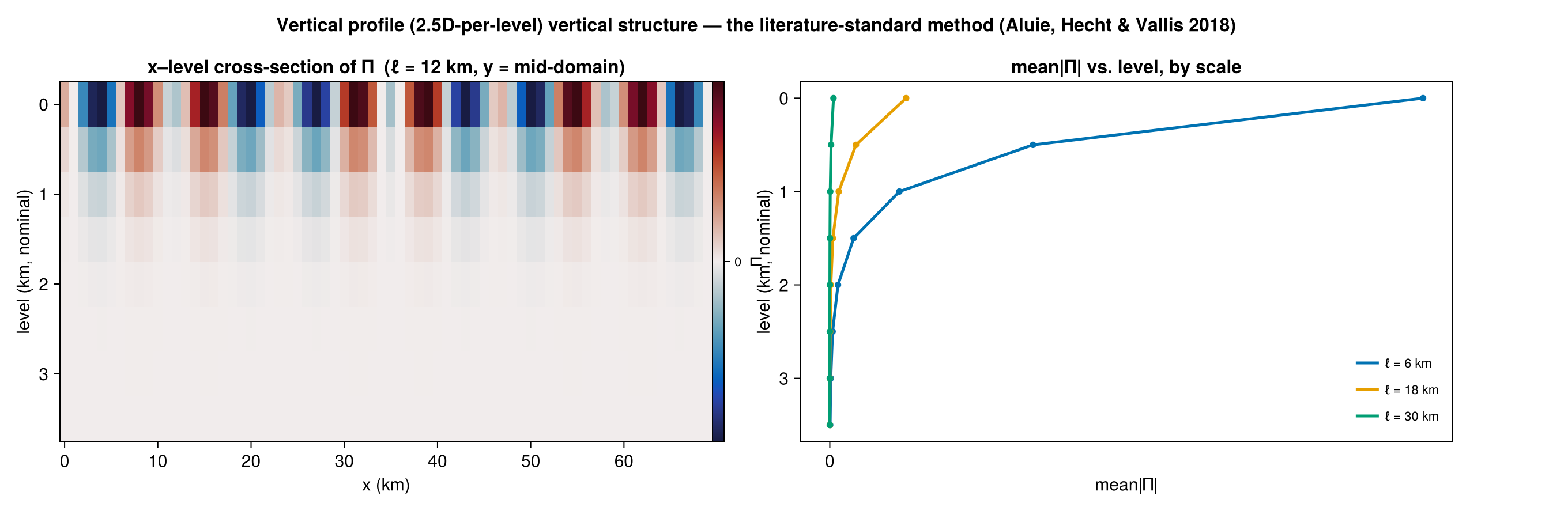
Vertical profile (2.5D per-level) vertical structure
Cartesian domain — flux at one scale and across scales
using CoarseGrainingEnergyFluxes: CoarseGrainingEnergyFluxes as CGEF
using FlowGeometries: FlowGeometries as FG

dx = 1_000.0; N = 100                       # 100 km × 100 km patch, 1 km spacing
geom = FG.Geometry.CartesianGeometry()
xs = collect(0.0:dx:(N - 1) * dx)
ys = collect(0.0:dx:(N - 1) * dx)
grid = FG.Grids.StructuredGrid(geom, xs, ys)   # no mask ⇒ `AllActive`; see below to exclude cells

u = randn(N, N); v = randn(N, N)            # replace with your data

# Π at a single 10 km scale.
Π = zeros(N, N)
CGEF.Diagnostics.compute_Π!(Π, u, v, nothing, grid, CGEF.TopHatKernel(), 10_000.0)

# Multi-scale sweep (plan reuse handled internally).
scales = collect(5e3:5e3:50e3)
result = CGEF.coarse_grain(u, v, grid; scales = scales, kernel = CGEF.TopHatKernel(),
                           spectrum = CGEF.Diagnostics.NoSpectrum())
@view result.Π[:, :, 3]      # flux map at scales[3] — result.Π is a stacked (Nx,Ny,Nscales) array
result.cumulative_energy     # ½ρ₀⟨|ū_ℓ|²⟩ per scale (Sadek–Aluie Eq. 15)
result.wavenumber            # k_ℓ = L/ℓ

# The spectral density needs a kernel whose |Ĝ|² is monotone — see the note below.
spec = CGEF.coarse_grain(u, v, grid; scales = scales, kernel = CGEF.GaussianKernel())
spec.filtering_spectrum # Ẽ(k_ℓ) density (Eq. 14)TopHatKernel's |Ĝ|² is not monotone decreasing, so Sadek & Aluie (2018) eq. 21 does not apply and the spectral density may dip below zero. That condition is sufficient, not necessary — the top-hat's |Ĝ|² falls to zero at kℓ ≈ 7.66 and then climbs back to only 0.0175 at kℓ ≈ 10.27 (the first Airy sidelobe; later ones reach 0.0042 and 0.0016), so the violation is confined to the far sub-filter tail at under 2% of the DC value. The density is usually perfectly usable and the default merely declines to vouch for it. Three ways forward, per Diagnostics.AbstractSpectrumPolicy:
| you want | pass |
|---|---|
| a density you don't have to check | kernel = CGEF.GaussianKernel() |
| the top-hat's density, sign checked yourself | spectrum = CGEF.Diagnostics.ForceSpectrum() |
only Π and cumulative_energy | spectrum = CGEF.Diagnostics.NoSpectrum() |
Π and cumulative_energy are unaffected by the choice — neither depends on the condition. See Kernels.transfer_monotone.
Spherical domain with a mask
using CoarseGrainingEnergyFluxes: CoarseGrainingEnergyFluxes as CGEF
using FlowGeometries: FlowGeometries as FG

geom = FG.Geometry.SphericalGeometry(6.371e6)
lon = deg2rad.(collect(0.0:0.25:359.75))
lat = deg2rad.(collect(-80.0:0.25:80.0))
grid = FG.Grids.StructuredGrid(geom, lon, lat)   # full-circle lon ⇒ periodic auto-detected
# u, v = load_velocity(...)

scales = collect(10e3:10e3:300e3)
result = CGEF.coarse_grain(u, v, grid; scales = scales, kernel = CGEF.TopHatKernel(),
                           spectrum = CGEF.Diagnostics.NoSpectrum())
The ZeroFill mask strategy (default) treats excluded cells as zeros, keeping the kernel position-independent so that filtering commutes with spatial derivatives — the property the Π budget is derived by. Pass mask_strategy = CGEF.Filtering.Deformable() to renormalize the kernel over active points near the boundary instead: that reproduces a constant field exactly there, but the kernel changes shape, so it neither commutes with derivatives nor conserves the domain average. Either way, points within ≈ℓ of a mask boundary are contaminated — see Filtering.filter_field! for the measured artifacts.
Curvilinear (model-native) grids
CurvilinearGrid needs no rectilinear axis assumption at all — every point carries its own (x, y), and derivatives/filtering/Π all work directly off the 2D coordinate arrays via a per-point footprint and weighted-least-squares (WLSQ) gradients. A common source is a structured-grid ocean/atmosphere model's curvilinear cell-center grid; here's a synthetic sheared/rotated example:
using CoarseGrainingEnergyFluxes: CoarseGrainingEnergyFluxes as CGEF
using FlowGeometries: FlowGeometries as FG

N = 60; dx = 2_000.0
geom = FG.Geometry.CartesianGeometry()
i = collect(0.0:(N - 1)); j = collect(0.0:(N - 1))
θ = deg2rad(15.0); shear = 0.3                       # rotate + shear a rectilinear index grid
x = [dx * (ii * cos(θ) - jj * shear * sin(θ)) for ii in i, jj in j]
y = [dx * (ii * sin(θ) + jj * (1 + shear * cos(θ))) for ii in i, jj in j]
grid = FG.Grids.CurvilinearGrid(geom, x, y)     # exact corner-based cell areas, auto-reconstructed

u = randn(N, N); v = randn(N, N)
result = CGEF.coarse_grain(u, v, grid; scales = collect(10e3:10e3:60e3),
                           kernel = CGEF.TopHatKernel(), spectrum = CGEF.Diagnostics.NoSpectrum())
Scattered / unstructured point clouds
UnstructuredGrid is the full pipeline for genuinely scattered observations (moorings, drifters, along-track altimetry): k-d tree neighbor search and Voronoi cell areas at construction time, WLSQ gradients over that adjacency, and both filtering methods. RealSpace() is the default, as on every other grid: the compact kernel applied exactly as written, through a gather over each point's metric ball, which holds next to a boundary or a masked region. Pass method = CGEF.Filtering.Spectral() for the transform — exact for a band-limited field on a homogeneous domain, and O(n log n).
using CoarseGrainingEnergyFluxes: CoarseGrainingEnergyFluxes as CGEF
using FlowGeometries: FlowGeometries as FG
using NearestNeighbors: NearestNeighbors        # enables k-d tree neighbor search
using DelaunayTriangulation: DelaunayTriangulation  # enables exact Voronoi cell areas (Cartesian)
using FINUFFT: FINUFFT                          # enables scattered-Cartesian spectral filtering

npts = 2_000
geom = FG.Geometry.CartesianGeometry()         # a placeholder — UnstructuredGrid has no fixed spacing
x = 100_000.0 .* rand(npts)
y = 100_000.0 .* rand(npts)
grid = FG.Grids.UnstructuredGrid(geom, x, y; k = 8)   # k-nearest adjacency + auto Voronoi areas

u = randn(npts); v = randn(npts)
Π = zeros(npts)
CGEF.Diagnostics.compute_Π!(Π, u, v, nothing, grid, CGEF.GaussianKernel(), 8_000.0)
For scattered spherical observations, build grid with FG.Geometry.SphericalGeometry(R) instead and load Quickhull (Voronoi areas) and NUFSHT (spectral filtering) in place of DelaunayTriangulation/ FINUFFT.
Sphere pixelizations: ring, cubed-sphere, healpix, icosahedral, Yin–Yang
A model that stores one value per cell and names that cell by a single index is served by the same engine as a scattered point cloud: a gather over each cell's own metric ball, with each cell weighted by its own area. The grid declares Grids.cell_address(grid) === Grids.FlatCells() and the whole pipeline follows — filtering, gradients, compute_Π!, a scale sweep, every execution backend, and the tensor diagnostics (tau_decomposition, tracer_variance_flux, vorticity, enstrophy_flux, and on a Cartesian metric compute_Π_strain_convergence, compute_Π_decomposed and compressible_flux). Nothing in the call names the layout.
using CoarseGrainingEnergyFluxes: CoarseGrainingEnergyFluxes as CGEF
using FlowGeometries: FlowGeometries as FG

geom = FG.Geometry.SphericalGeometry(6.371e6)

grid = FG.Grids.HEALPixGrid(geom, 64)               # 12·64² = 49,152 equal-area pixels
# grid = FG.Grids.CubedSphereGrid(geom, 48)         # 6 faces of 48²
# grid = FG.Grids.IcosahedralGrid(geom, 32)         # 10·32² + 2 vertices
# grid = FG.Grids.YinYangGrid(geom, 192, 96)        # two overlapping lat-lon panels
# grid = FG.Grids.RingGrid(geom, FG.SphericalSampling.ReducedGaussianSampling(nlon_per_ring))

n = length(FG.Grids.mask(grid))
u = randn(n); v = randn(n)                          # one value per cell, in the grid's own ordering

Π = zeros(n)
CGEF.Diagnostics.compute_Π!(Π, u, v, nothing, grid, CGEF.GaussianKernel(), 300e3)

result = CGEF.coarse_grain(u, v, grid; scales = collect(100e3:100e3:600e3),
                           kernel = CGEF.GaussianKernel(),
                           spectrum = CGEF.Diagnostics.NoSpectrum())
Pass mask = <Vector{Bool}> to any of these constructors for a regional or land-masked domain; the mask strategies behave as they do everywhere else. These layouts store no coordinate arrays — a cell's position, neighbours and area are arithmetic in the resolution parameter — so Grids.coordinates is unavailable on them and check_setup reports no axis spacing.
True 3D volumetric flux (Cartesian and spherical)
Distinct from the vertical-profile method below: a true 3D StructuredGrid filters in all three directions with one kernel and computes the genuinely coupled 9-component strain/stress contraction — the right tool for homogeneous/isotropic turbulence, not the standard large-scale thin-layer level-stacking approach.
using CoarseGrainingEnergyFluxes: CoarseGrainingEnergyFluxes as CGEF
using FlowGeometries: FlowGeometries as FG

# Cartesian: (x, y, z) all uniform Range axes.
N = 24; dx = 500.0
geom = FG.Geometry.CartesianGeometry()
x = collect(0.0:dx:(N - 1) * dx); y = copy(x); z = copy(x)
grid = FG.Grids.StructuredGrid(geom, x, y, z)

u = randn(N, N, N); v = randn(N, N, N); w = randn(N, N, N)
Π = zeros(N, N, N)
CGEF.Diagnostics.compute_Π!(Π, u, v, w, grid, CGEF.TopHatKernel(), 5_000.0)

# Spherical volumetric shell: (lon, lat, radius); Nz ≥ 2 is required (else use the 2D constructor).
R = 6.371e6
sgeom = FG.Geometry.SphericalGeometry(R)
lon = deg2rad.(collect(0.0:2.0:358.0)); lat = deg2rad.(collect(-80.0:2.0:80.0))
r = collect((R - 2000.0):500.0:R)                     # 5 levels spanning the top 2 km
sgrid = FG.Grids.StructuredGrid(sgeom, lon, lat, r)
Vertical profile (2.5D per-level) vertical structure
The literature-standard method (Aluie, Hecht & Vallis 2018): run the existing 2D/2.5D compute_Π! independently at each vertical level of a 3D (x, y, z) array and stack the profile — not to be confused with the coupled true-3D method above.
using CoarseGrainingEnergyFluxes: CoarseGrainingEnergyFluxes as CGEF
using FlowGeometries: FlowGeometries as FG

geom = FG.Geometry.CartesianGeometry()
N = 80; Nz = 6
xs = collect(0.0:1_000.0:(N - 1) * 1_000.0)
grid = FG.Grids.StructuredGrid(geom, xs, xs)    # a 2D grid — z is a third array axis

u = randn(N, N, Nz); v = randn(N, N, Nz)                 # (x, y, z)
scales = collect(5e3:5e3:30e3)
batch = CGEF.coarse_grain_profile(u, v, grid; scales = scales, kernel = CGEF.TopHatKernel(),
                                  spectrum = CGEF.Diagnostics.NoSpectrum())
# The vertical axis is a batch axis, so it is TRAILING: Π is (x, y, scale, level).
batch.Π[:, :, 3, :]                 # flux profile at scales[3], all Nz levels
batch.cumulative_energy[3, :]       # per-level cumulative energy at scales[3]
batch.slices[2].Π                   # level 2's own (x, y, scale) result, a zero-copy view
Execution backends (real-space RealSpace)
The backend only changes how the same footprint convolution is evaluated — results are identical. Every backend reuses a footprint/plan built once per (grid, kernel, scale), not rebuilt per call.
using OhMyThreads: OhMyThreads          # enables ThreadedBackend (2D row-parallel + 1D/3D point-parallel)
result = CGEF.coarse_grain(u, v, grid; scales = scales, spectrum = CGEF.Diagnostics.NoSpectrum(), backend = CGEF.ComputationalBackends.ThreadedBackend())

using KernelAbstractions: KernelAbstractions   # enables GPUBackend (2D grids only)
# Takes the device to run on — `KernelAbstractions.CPU()` here, `CUDABackend()`/`ROCBackend()` on a GPU.
result = CGEF.coarse_grain(u, v, grid; scales = scales, spectrum = CGEF.Diagnostics.NoSpectrum(),
                           backend = CGEF.ComputationalBackends.GPUBackend(KernelAbstractions.CPU()))

using MPI: MPI                          # enables MPIBackend (2D grids; requires MPI.Init() first)
result = CGEF.coarse_grain(u, v, grid; scales = scales, spectrum = CGEF.Diagnostics.NoSpectrum(), backend = CGEF.ComputationalBackends.MPIBackend())

# AutoBackend (default) picks ThreadedBackend when Threads.nthreads() > 1, else SerialBackend.MPIBackend's real multi-rank behavior (round-robin row decomposition + Allreduce!) is only meaningfully exercised under mpiexec -n P; see test/mpi_runtests.jl for a runnable reference.
Planning a sweep once instead of once per scale
A filter plan splits by how often each part changes: what the grid fixes (transform objects, measure prefix scans, a scattered point sort), what the scale fixes (tap tables, Ĝ(ℓ), the reciprocal window mass), and transient scratch. plan_filter builds one of each for a single scale; Filtering.plan_filter_sweep builds the grid part and the scratch once for a whole sweep and gives each scale only its own tables.
scales = collect(10e3:10e3:80e3)
family = CGEF.Filtering.plan_filter_sweep(grid, CGEF.TopHatKernel(), scales)

# The allocating entry point sizes the result and a workspace; hand both, plus the family, to the
# in-place one for every later timestep.
result = CGEF.coarse_grain(u, v, grid; scales = scales, spectrum = CGEF.Diagnostics.NoSpectrum())
ws = CGEF.Diagnostics.ΠWorkspace(grid)
for t in 2:nt
    CGEF.coarse_grain!(result, us[t], vs[t], grid; scales = scales,
                       filter_plans = family, workspace = ws,
                       spectrum = CGEF.Diagnostics.NoSpectrum())
end
A FilterPlanFamily is an AbstractVector of the per-scale plans, so it can be indexed, iterated, and passed anywhere a plain vector of plans was. coarse_grain builds one internally for a one-shot sweep; coarse_grain! is the entry point that takes a prebuilt one.
Because the scales of one family share a scratch buffer, a family may not be applied from several tasks at once. Give each concurrent worker its own — the batch and slice drivers already do.
Choosing the evaluator: AutoMethod()
RealSpace() computes the direct sum. AutoMethod() picks the fastest engine that computes the same convolution, which on some grids means evaluating it by transform:
# Global sphere + a radial kernel: each latitude band becomes a circular convolution along longitude.
res_fast = CGEF.coarse_grain(u, v, sphere_grid; scales = scales, kernel = CGEF.GaussianKernel(),
                             method = CGEF.Filtering.AutoMethod(),
                             spectrum = CGEF.Diagnostics.NoSpectrum())

# Which engine did that pick, and what would RealSpace() have used?
CGEF.check_setup(sphere_grid, CGEF.GaussianKernel(), 800e3; method = CGEF.Filtering.AutoMethod())
CGEF.check_setup(sphere_grid, CGEF.GaussianKernel(), 800e3)   # notes that AutoMethod would be faster
These are the same compact kernel with the same weights, so they agree with the direct sum to round-off rather than exactly — which is why RealSpace() remains the default. Neither is method = Spectral(): no transfer function is sampled and no spherical-harmonic truncation happens.
Workspaces sized to what you asked for
Each in-place diagnostic takes a workspace holding only the buffers its configuration can reach:
ws  = CGEF.Diagnostics.ΠWorkspace(grid)                  # 2-D flux, no vertical component
wsw = CGEF.Diagnostics.ΠWorkspace(grid; has_w = true)    # 2.5-D: adds the vertical-component buffers
ew  = CGEF.Diagnostics.EnergyWorkspace(grid)             # E(ℓ) reads only filtered velocity: 2 buffers

CGEF.Diagnostics.compute_Π!(Π, u, v, nothing, grid, kernel, ℓ; workspace = ws)
CGEF.Diagnostics.cumulative_energy!(E, u, v, nothing, grid, kernel, scales; workspace = ew)
has_w must be given at construction, because the buffers have to exist before the first call — a workspace built without them refuses a w rather than returning a wrong answer. Spherical and true-3-D grids always carry the full set, since the spherical branch works in three planetary-Cartesian components whether or not a vertical velocity was supplied.
Spectral filtering (method = Spectral())
Spectral filtering multiplies by Ĝ(k) and is selected by the grid type (FFTW / FINUFFT / FastSphericalHarmonics / NUFSHT). It requires a homogeneous (periodic / global) domain, but a partial mask is supported — ZeroFill/Deformable work exactly as they do for RealSpace() (normalized convolution, evaluated in Fourier/spherical-harmonic space). GaussianKernel/SharpSpectralKernel work with no extra dependency; TopHatKernel needs using SpecialFunctions (for its exact planar Bessel-J₁ transfer function — the spherical-cap analog needs no extra dependency).
using FlowGeometries: FlowGeometries as FG
using FFTW: FFTW                       # uniform periodic Cartesian
N = 128; dx = 1.0
geom = FG.Geometry.CartesianGeometry()
x = collect(0.0:dx:dx*(N - 1))
grid = FG.Grids.StructuredGrid(geom, x, x; periodic = (true, true))

out = zeros(N, N)
CGEF.Filtering.filter_field!(out, u, grid, CGEF.GaussianKernel(), 4.0; method = CGEF.Filtering.Spectral())
Scattered Cartesian points use FINUFFT on an UnstructuredGrid{Cartesian}; uniform spherical grids use FastSphericalHarmonics on a StructuredGrid{Spherical}; scattered spherical points use NUFSHT on an UnstructuredGrid{Spherical}. In every case the call is the same filter_field!(…; method = CGEF.Filtering.Spectral()) — only the grid type differs.
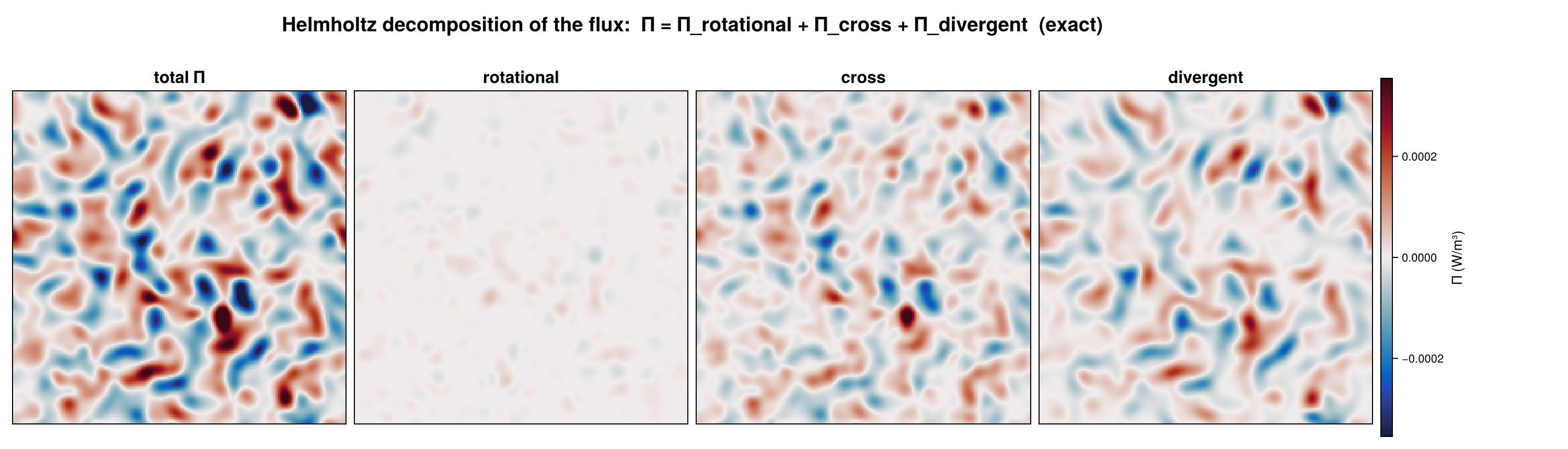
Rotational / divergent (Helmholtz) flux decomposition
Pass the rotational (solenoidal) velocity from a Helmholtz solver (HelmholtzDecomposition.jl); the divergent part is taken as the complement. Both the strain and the stress are split before contracting (see Theory), giving three exact channels rather than a one-sided approximation.
using CoarseGrainingEnergyFluxes: CoarseGrainingEnergyFluxes as CGEF
# u_rot, v_rot = HelmholtzDecomposition.rotational_part(u, v, grid)

dec = CGEF.Diagnostics.compute_Π_decomposed(u, v, u_rot, v_rot, grid, CGEF.TopHatKernel(), 20_000.0)
dec.total        # == compute_Π! full flux
dec.rotational   # Π_RR   (rotational → rotational)
dec.cross        # Π_X    (every interaction / "stimulated cascade" term)
dec.divergent    # Π_DD   (divergent → divergent)      dec.rotational .+ dec.cross .+ dec.divergent ≈ dec.total
The true-3D method has the same signature with w/w_rot added, on a Cartesian volume or a spherical shell.
On a spherical grid the call is identical. The three stress pieces are formed as generalized second moments in planetary-Cartesian coordinates and rotated back to the local frame, and each part's strain carries the frame's tanφ/R curvature terms, so dec.total still equals compute_Π! — the suite asserts it. Pass SphericalPiDecomposedWorkspace(grid) to compute_Π_decomposed! to reuse the buffers across a sweep.
Tracer / buoyancy variance flux
# θ is any tracer (buoyancy b = -g ρ'/ρ₀ gives the APE-related transfer).
Πθ = CGEF.Diagnostics.tracer_variance_flux(u, v, θ, grid, CGEF.TopHatKernel(), 20_000.0)
A true-3D method exists too (tracer_variance_flux(u, v, w, θ, grid, kernel, scale)). On a spherical grid the velocity is rotated to planetary Cartesian before filtering and the subfilter tracer flux rotated back to east/north(/radial), the same convention compute_Π! uses.
Stress decomposition (Leonard / Cross / Reynolds)
d = CGEF.Diagnostics.tau_decomposition(u, v, grid, CGEF.TopHatKernel(), 20_000.0)
d.L.xx; d.C.xy; d.R.yy        # d.L + d.C + d.R == τ exactly
On a spherical grid, xx/xy/yy are local east/north components (the moments are taken in planetary-Cartesian coordinates, then rotated back — see Theory).
Add w for the true-3-D split, on a Cartesian volume or a spherical shell. Each tensor then comes back with all six independent components, (; xx, xy, xz, yy, yz, zz), and L + C + R = τ holds componentwise:
d3 = CGEF.Diagnostics.tau_decomposition(u, v, w, grid3d, CGEF.GaussianKernel(), 20_000.0)
d3.L.xz; d3.C.yz; d3.R.zz
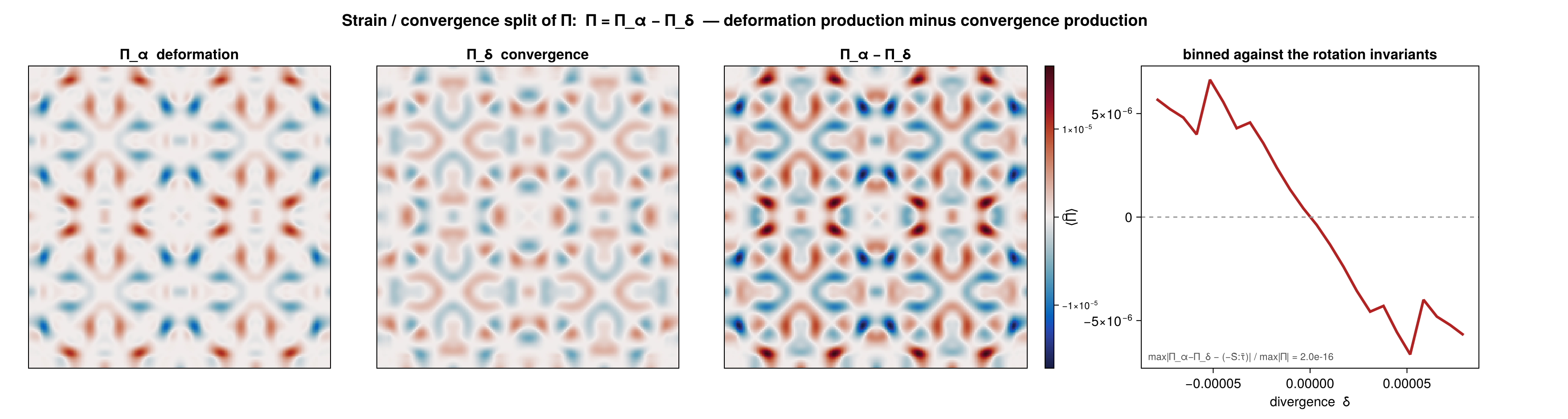
Strain / convergence decomposition of Π
The same flux split by diagonalizing the filtered strain instead of decomposing the velocity (Srinivasan, Barkan & McWilliams 2023). Π_α is deformation production, Π_δ the frontogenetic convergence term that vanishes for a non-divergent field.
d = CGEF.Diagnostics.compute_Π_strain_convergence(u, v, grid, CGEF.TopHatKernel(), 20_000.0)
d.total                       # == compute_Π! to round-off; the suite asserts it
d.strain                      # Π_α — deformation / shear production
d.convergence                 # Π_δ — convergence production (zero if ∇·u = 0)
d.divergence                  # δ̄, a rotation invariant: the natural axis to bin the flux against
d.strain_magnitude            # ᾱ, likewise

# Reuse across timesteps or scales without reallocating:
ws = CGEF.Diagnostics.PiStrainWorkspace(grid)
CGEF.Diagnostics.compute_Π_strain_convergence!(ws, u, v, grid, ker, ℓ;
                                               filter_plan = plan, deriv_plan = dplan)
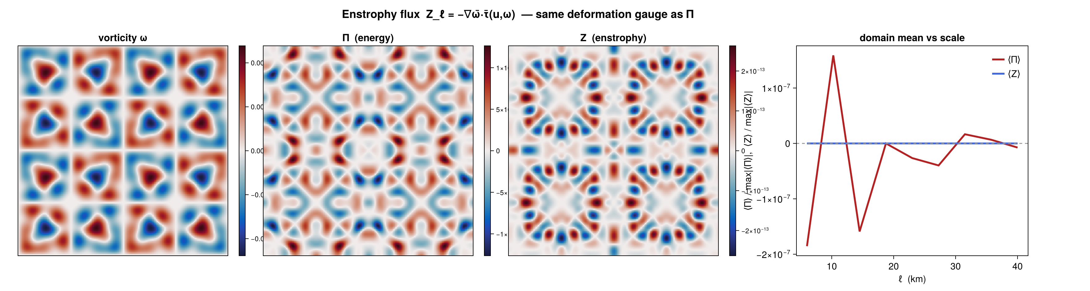
Enstrophy flux
The enstrophy analogue of Π, in the same (deformation) gauge — in 2-D turbulence this cascades forward while Π cascades inverse, so the two are read together.
ω = CGEF.Diagnostics.vorticity(u, v, grid)            # ∂v/∂x − ∂u/∂y
Z = CGEF.Diagnostics.enstrophy_flux(u, v, grid, CGEF.GaussianKernel(), 20_000.0)

ws = CGEF.Diagnostics.EnstrophyFluxWorkspace(grid)    # zero-allocation repeat
CGEF.Diagnostics.enstrophy_flux!(Z, ws, u, v, grid, ker, ℓ; filter_plan = plan, deriv_plan = dplan)
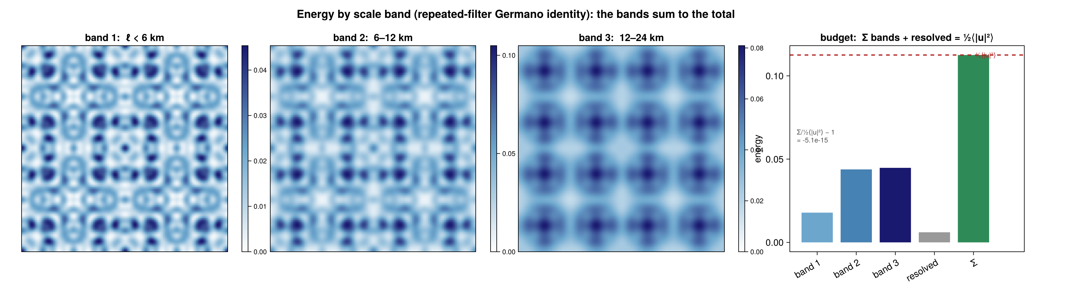
Energy by scale band
The repeated-filter Germano identity, which splits the kinetic energy into bands that sum to the total — unlike band-passing the velocity, whose cross terms have indefinite sign.
# `scales` ASCENDING: band n is what the n-th, progressively coarser, filter removes.
# `maps = true` adds the pointwise fields; without it only the scalars are formed.
r = CGEF.Diagnostics.band_energies(u, v, grid, CGEF.GaussianKernel(), [3e3, 6e3, 12e3];
                                   maps = true)
r.bands                       # domain-mean energy per band
r.resolved                    # what is left above the coarsest scale
r.total                       # == ½⟨|u|²⟩ exactly on a periodic, unmasked grid
r.band_maps[2]                # the pointwise map for band 2
Use a non-negative kernel here: band energies are variances, and they are pointwise positive only if the kernel is. The identity is exact on a periodic unmasked domain and carries an O(ℓ/L) residual wherever the footprint truncates — see Diagnostics.band_energies for the measured numbers.
Visualization (CairoMakie extension)
using CairoMakie: CairoMakie               # provides plot_Π_map / plot_spectrum methods
result = CGEF.coarse_grain(u, v, grid; scales = collect(10e3:10e3:100e3),
                           kernel = CGEF.GaussianKernel())   # a spectrum-admissible kernel

fig1 = CGEF.plot_Π_map(result, 3, grid)               # flux map at scales[3]
fig2 = CGEF.plot_spectrum(result; which = :density)   # filtering spectral density Ẽ(k_ℓ)
fig3 = CGEF.plot_spectrum(result; which = :cumulative) # cumulative coarse KE vs ℓ