ScatteringTransforms.jl

A fast, generic Julia implementation of the wavelet scattering transform for 1D signals, 2D images, 3D volumes, and scalar fields on the sphere — with averaged and localized outputs, reduced descriptors, a dependency-free default plus pluggable fast backends, batching, threading, distributed/MPI, and GPU.

Why scattering?

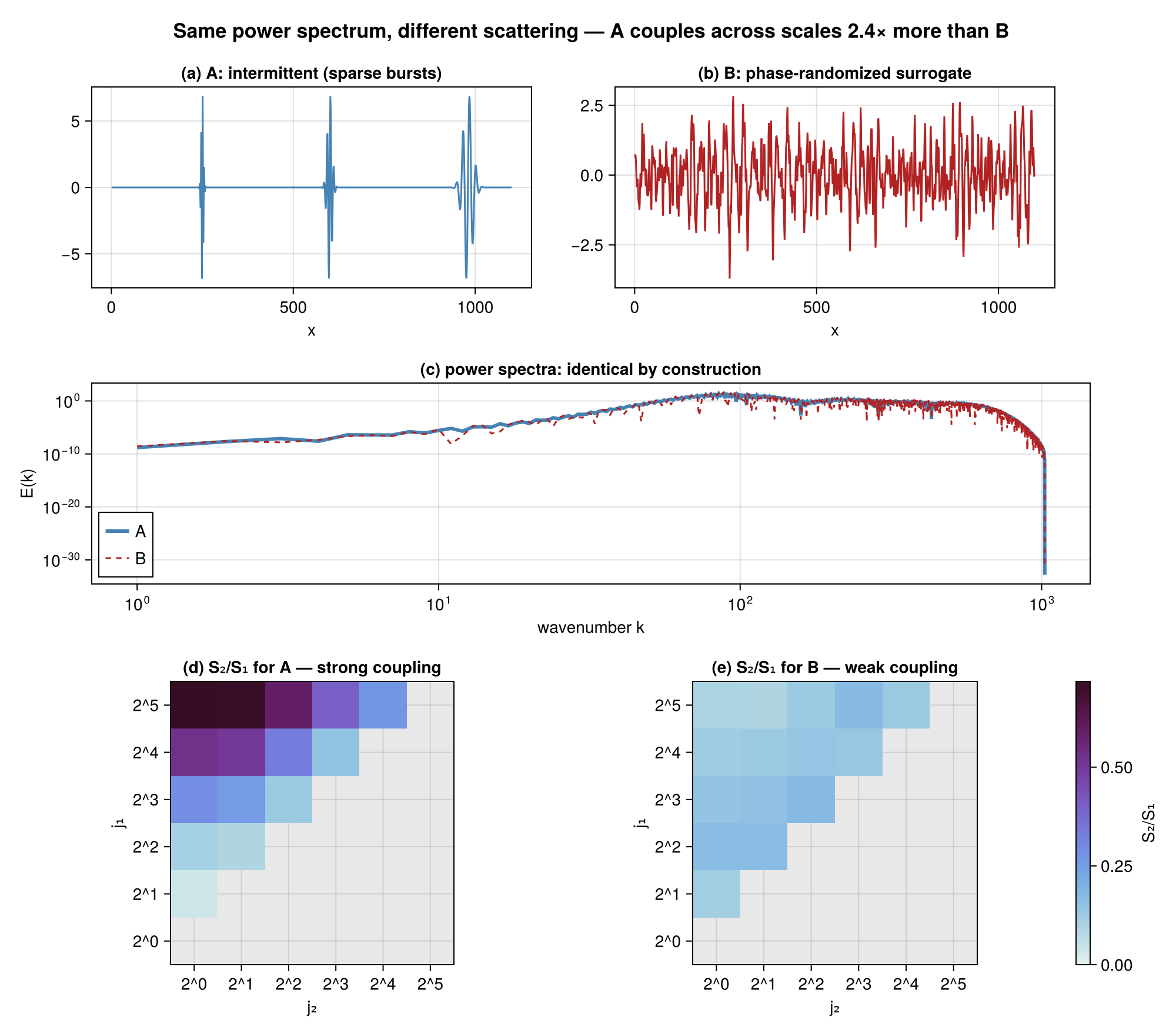
Two signals can share an identical power spectrum yet differ structurally. Scattering distinguishes them: an intermittent signal has strong cross-scale coupling S₂/S₁, while its phase-randomized Gaussian surrogate does not — though their power spectra and first-order S₁ are the same.

Features

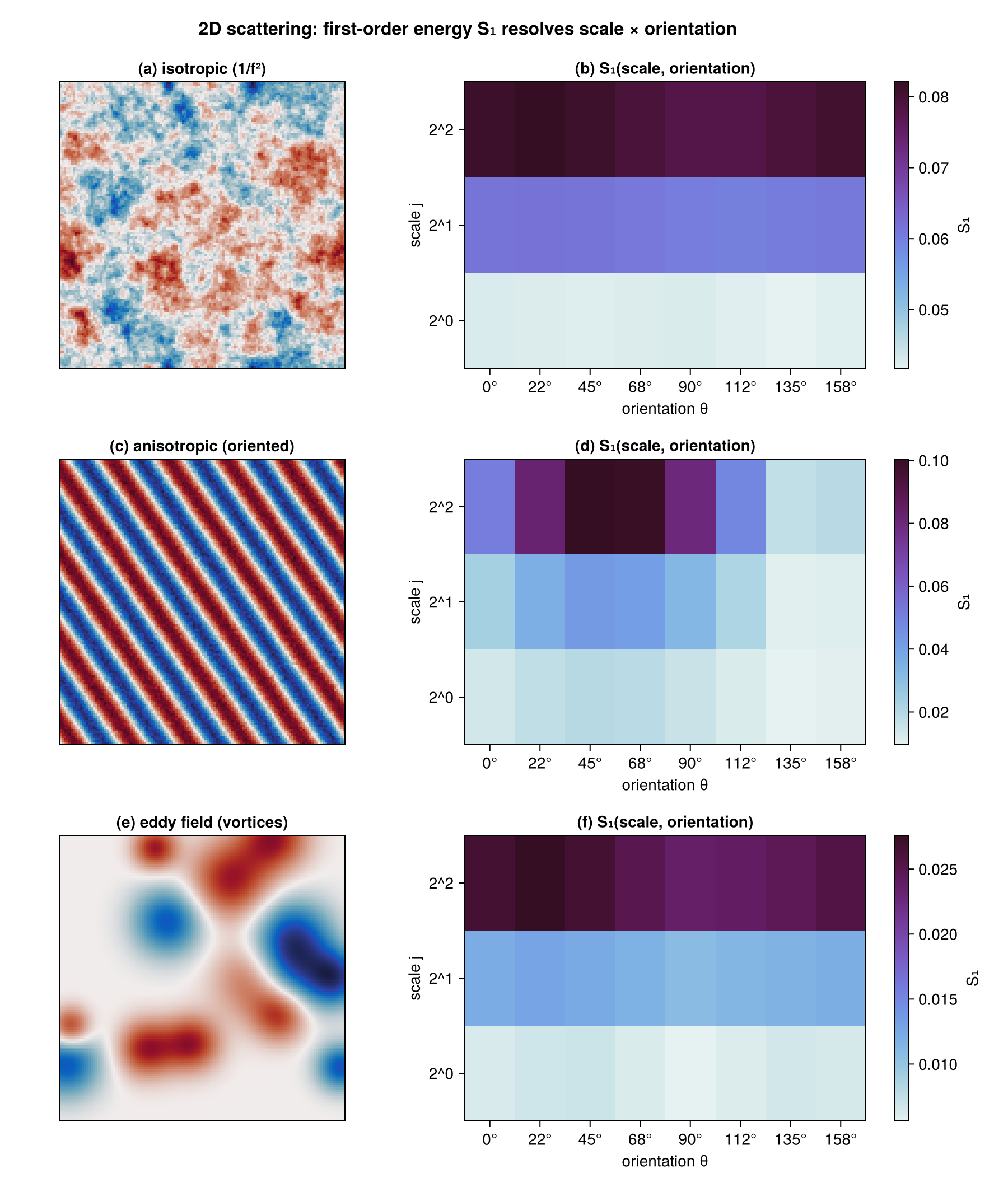
• Domains: 1D, 2D (oriented Morlet), 3D (oriented 3D Morlet), and spherical (S², smooth difference-of-Gaussians bands).
• Grid-support matrix: Cartesian × spherical, on uniform/structured and nonuniform/scattered sampling — gridded ScatteringTransform{1,2,3}D (FFT), scattered-planar scattered_planar_scattering (exact direct NUDFT), structured-sphere structured_spherical_scattering (fast SHT), scattered-sphere spherical_scattering (exact direct SHT). Every cell has an in-core, dependency-free default; FINUFFT / NUFSHT are optional fast paths selected via the spectral keyword.
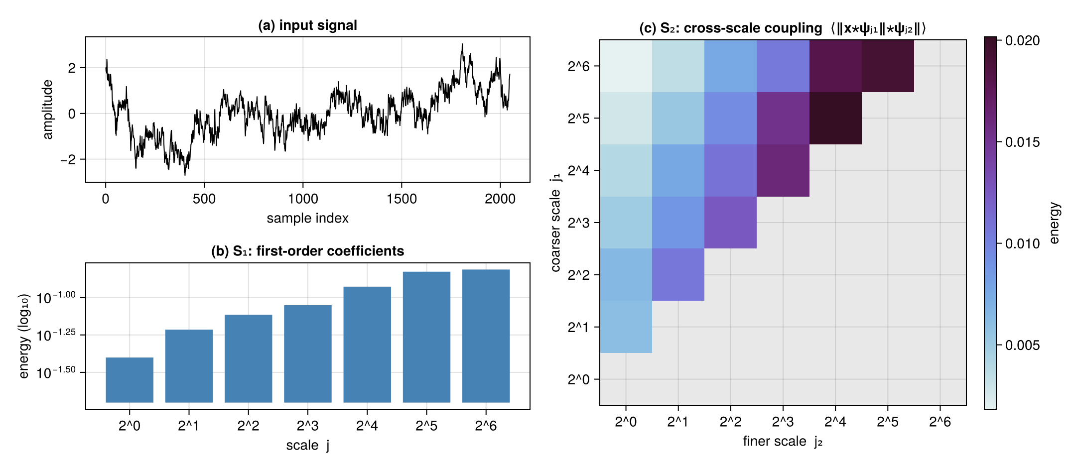
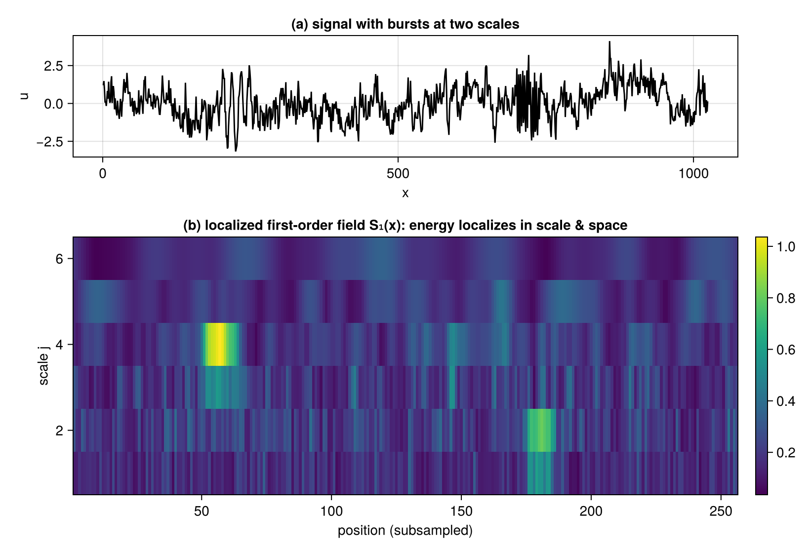
• Two outputs: globally-averaged coefficients st(x) and the localized (Mallat) field scattering_field(st, x) = (|U_p x| ⋆ φ_J)↓ (their spatial means agree by construction).
• Correct path structure: second order over strictly coarser scales, all orientation pairs.
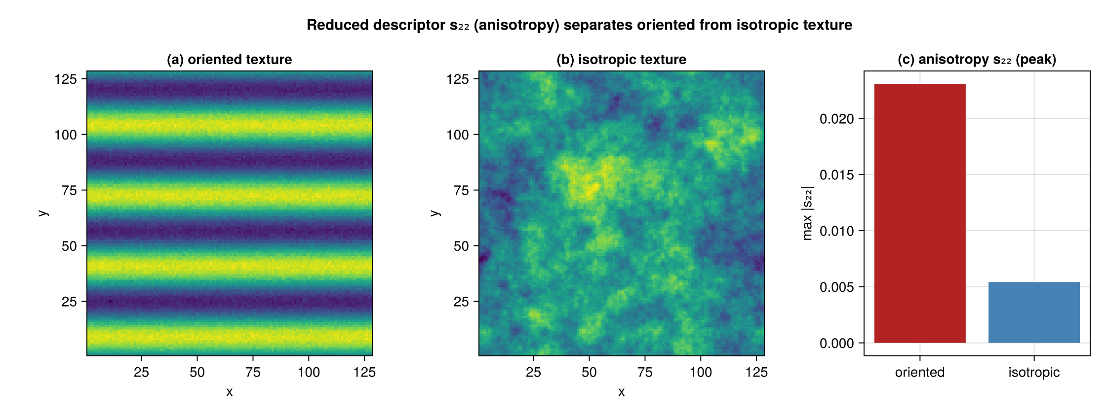
• Reduced descriptors: normalized_coefficients (S1/S0, S2/S1), log_coefficients, and 2D sparsity s₂₁ / anisotropy s₂₂ (compute_shape_sparsity).
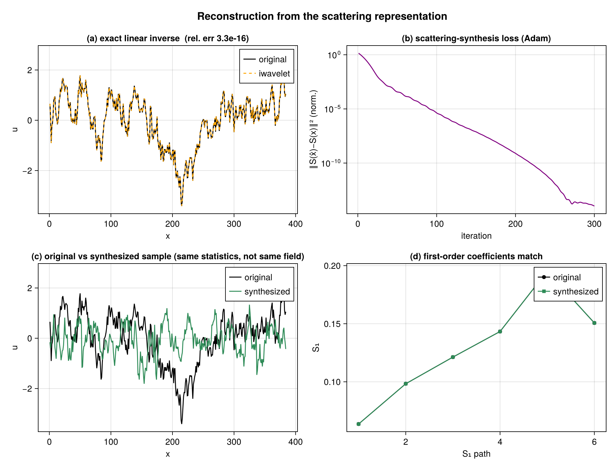
• Reconstruction: exact linear wavelet-frame inverse (wavelet_transform/iwavelet), phase retrieval (reconstruct_phase), and gradient-descent synthesize from coefficients (DifferentiationInterface extension, any ADTypes backend).
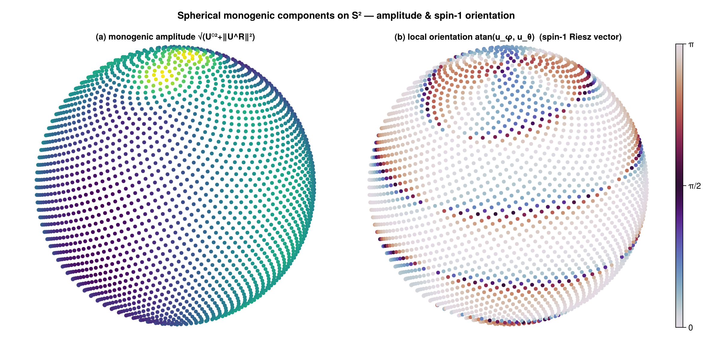
• Monogenic (Riesz) scattering: MonogenicScattering (1D/2D/3D) with the rotation-covariant monogenic amplitude + continuous orientation/phase (monogenic_components); on S², spherical_monogenic_scattering (amplitude) and spherical_monogenic_components (pointwise orientation/phase via the spin-1 Riesz vector).
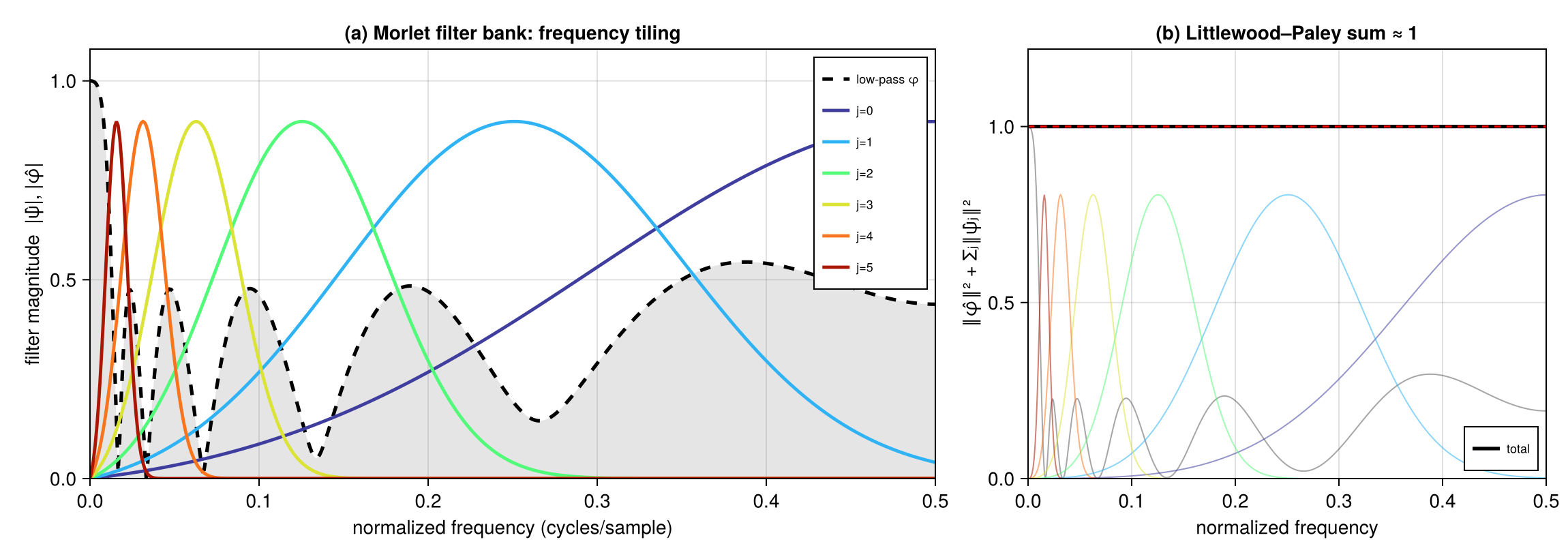
• Tight-frame filter bank: |φ|² + Σⱼ|ψⱼ|² ≡ 1 (non-expansive).
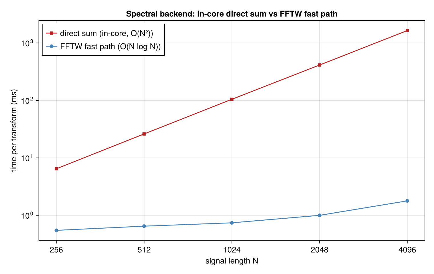
• Pluggable spectral backend: in-core direct-sum default; using FFTW → O(N log N) fast path (spectral = AutoSpectralBackend() | DirectSumSpectralBackend() | FFTSpectralBackend()).
• Scale: scattering_batch (one plan reused), ThreadedBackend (OhMyThreads), DistributedBackend/MPIBackend (parametric over the inner backend), GPUBackend (vendor-neutral KernelAbstractions: CUDA/ROCm/oneAPI/Metal, or KA.CPU()).
• Generic & type-stable: Float32/Float64, autodiff-friendly, GPU-array-ready hot path.

Quick start

Symbols live in submodules and are accessed via fully-qualified paths — the package intentionally does not re-export names into the top level (see the API Reference). Alias the package for brevity:

using ScatteringTransforms: ScatteringTransforms as ST
using FFTW: FFTW   # optional: loading it switches on the O(N log N) fast path automatically

# 1D
st = ST.Scattering1D.ScatteringTransform1D(1024, 8; Q=1, max_order=2)
c  = st(randn(1024))
ST.Coefficients.zeroth_order(c); ST.Coefficients.first_order(c); ST.Coefficients.second_order(c)

# 2D / 3D
c2 = ST.Scattering2D.ScatteringTransform2D((256, 256), 4; L=8)(randn(256, 256))
c3 = ST.Scattering3D.ScatteringTransform3D((32, 32, 32), 3; n_orient=6)(randn(32, 32, 32))

# localized field, reductions, batching
field = ST.ScatteringFields.scattering_field(st, randn(1024))   # per-path low-passed, subsampled maps
red   = ST.Reductions.normalized_coefficients(c)                # s1 = S1/S0, s2 = S2/S1
B     = ST.scattering_batch(st, randn(1024, 100))               # (coeffs × 100), one plan reused

Filter bank (tight frame)

1D and 2D scattering

Localized field and reductions

Reconstruction & synthesis

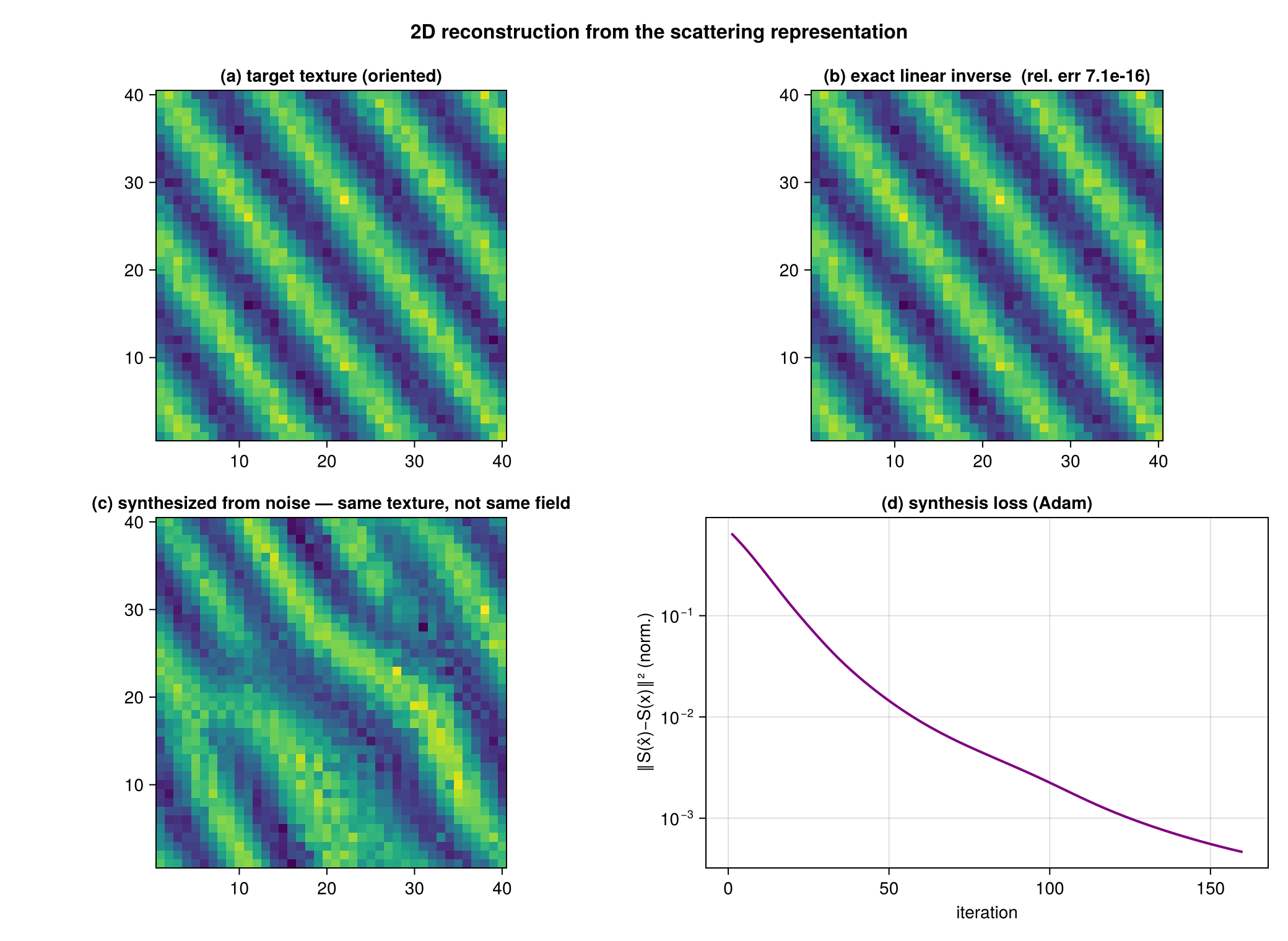
The complex (pre-modulus) wavelet layer is exactly invertible (iwavelet, machine precision); from the scattering coefficients, synthesize descends ‖S(x̂)−S(x)‖² (via DifferentiationInterface) to draw a new sample with matching multiscale statistics — in 1D and 2D.

using DifferentiationInterface: DifferentiationInterface
using Mooncake: Mooncake
using ADTypes: AutoMooncake
# exact linear inverse (machine precision)
x̂ = ST.Inverse.iwavelet(st, ST.Inverse.wavelet_transform(st, signal))
# coefficient synthesis from noise (a matching sample, not the original field)
res = ST.synthesize(st, signal; backend = AutoMooncake(), iters = 400)

Monogenic (Riesz) scattering

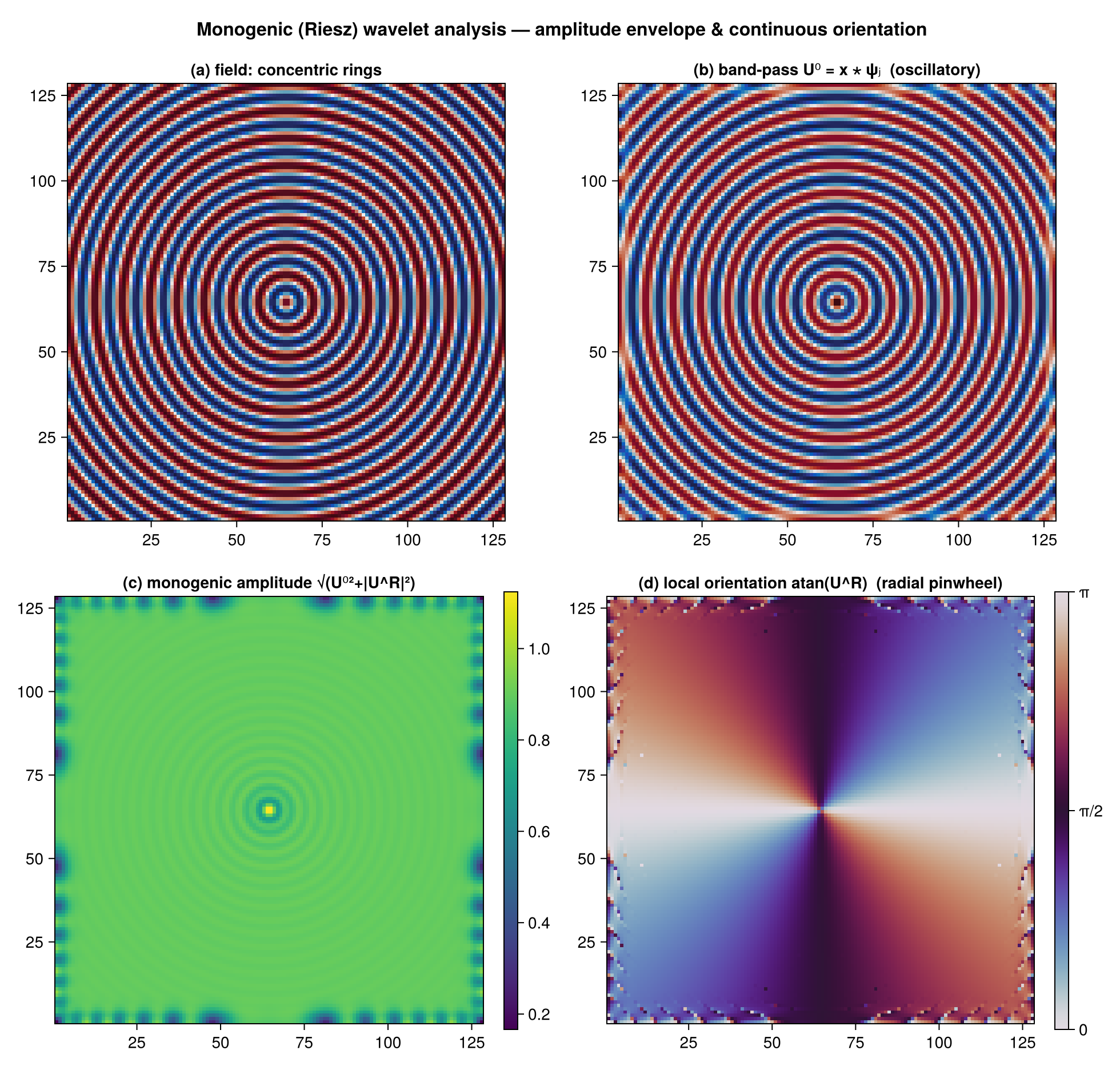
MonogenicScattering uses the rotation-covariant monogenic amplitude in place of the oriented modulus, and monogenic_components recovers the local amplitude envelope and a continuous orientation (not quantized into bins).

Nonuniform / scattered planar grids

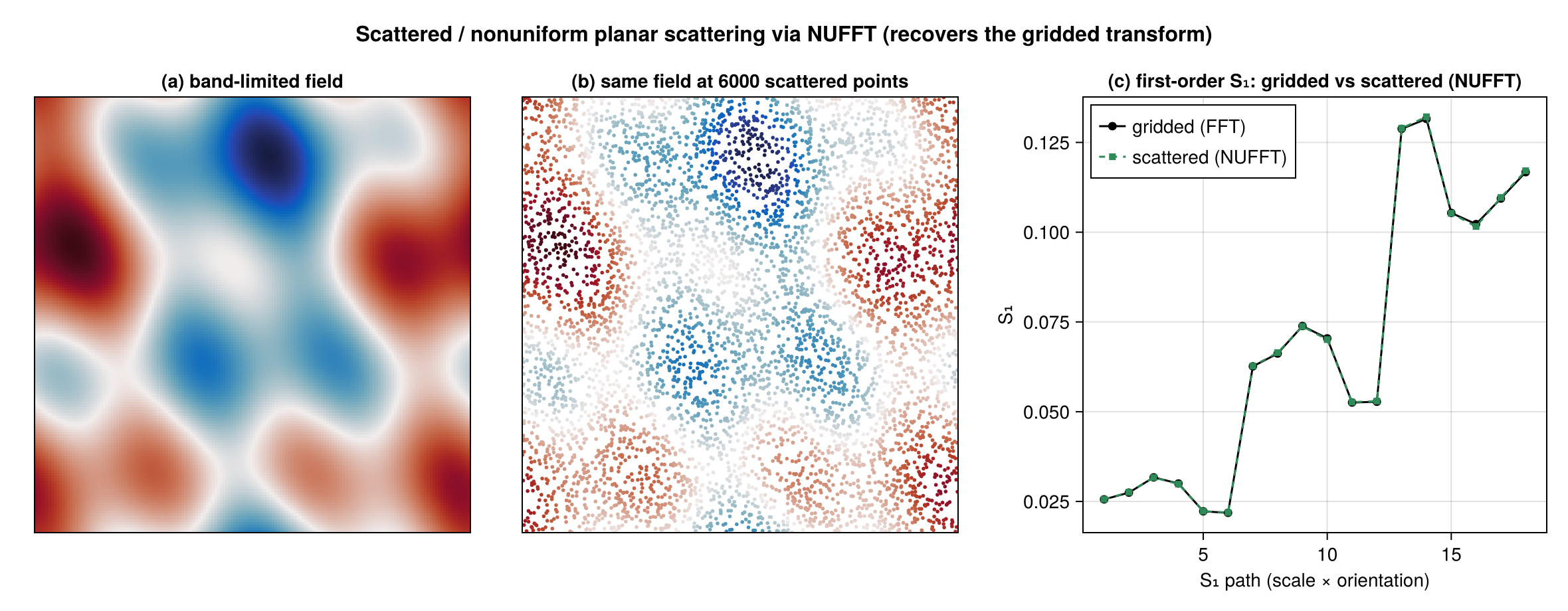
Off-lattice / gappy planar data is scattered onto a uniform Fourier mode grid by a nonuniform DFT (scattered_planar_scattering); on a uniform grid it reproduces the gridded FFT transform exactly. The default is an in-core exact direct NUDFT (no dependencies); using FINUFFT enables the faster NUFFT path via spectral = NUFFTSpectralBackend().

Spherical scattering

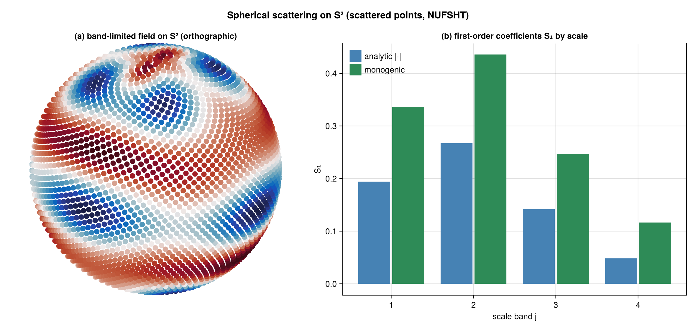
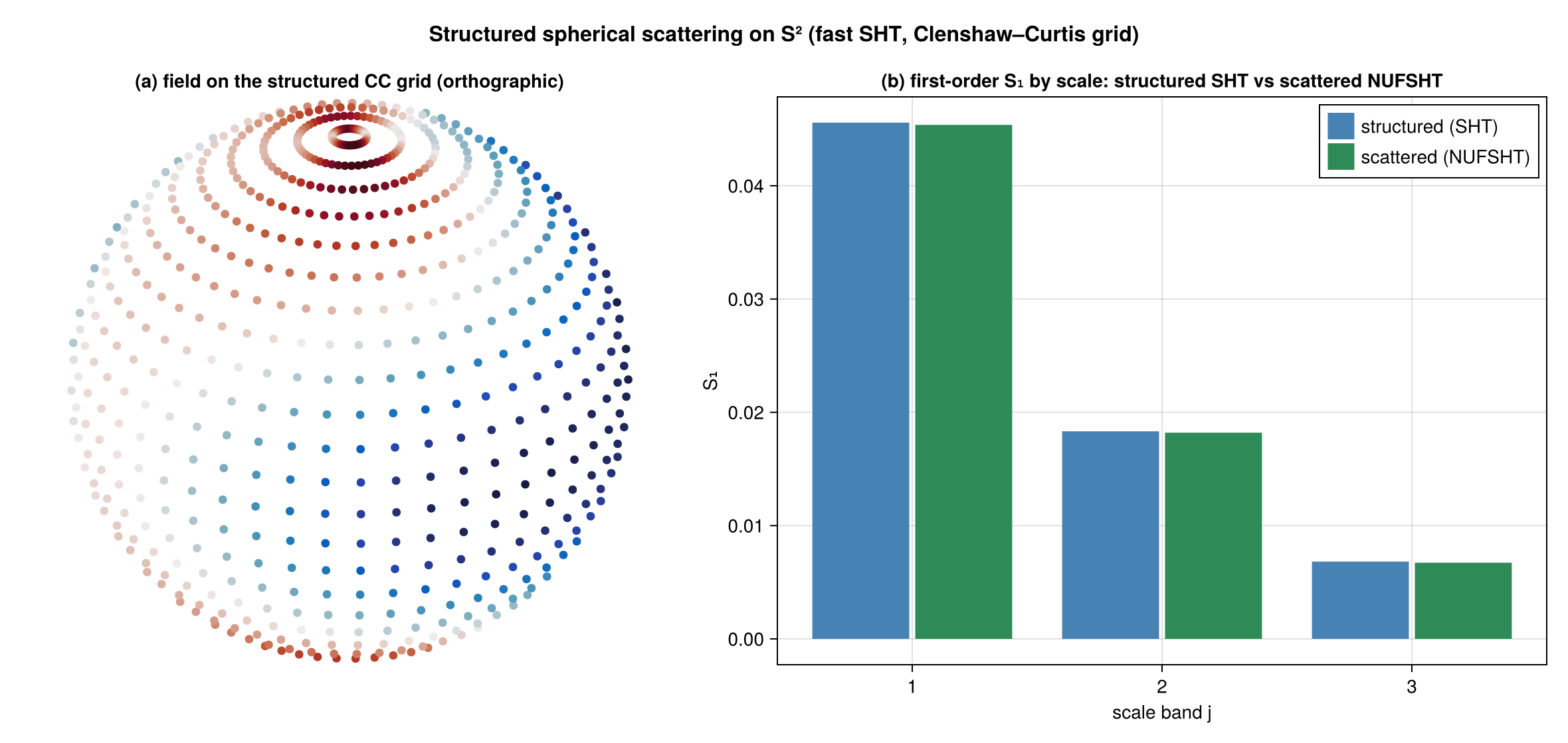
On S², both scattered points (spherical_scattering; in-core direct SHT by default, NUFSHT fast path when loaded) and a structured Clenshaw–Curtis grid (structured_spherical_scattering, fast SHT) give matching coefficients; the monogenic Riesz energy is computed with spin-0 transforms via a Bochner identity, and spherical_monogenic_components synthesizes the spin-1 Riesz vector for pointwise orientation/phase.

Backends & scale

The in-core direct-sum transform is dependency-free; loading FFTW selects an O(N log N) fast path automatically (identical results). scattering_batch reuses one plan/workspace across a stack; using OhMyThreads, using Distributed, or using MPI enable scattering_batch(ThreadedBackend(), …), DistributedBackend(…), and MPIBackend(…).

Documentation

• Theory — mathematical background
• API Reference — functions and types

Citation

@software{scatteringtransforms_jl,
  author = {Benjamin, Jordan},
  title = {ScatteringTransforms.jl: wavelet scattering in Julia},
  url = {https://github.com/jbphyswx/ScatteringTransforms.jl}
}