FlowGeometries.jl
Coordinate metrics, spherical samplings, and grid types for flow-field analysis on the plane and the sphere.
The package has no dependencies. Everything optional — spatial search, tessellation, sparse output, static vectors, FFT-based quadrature, device transfer, threading — arrives through package extensions, so you pay for exactly what you load.
Three orthogonal choices
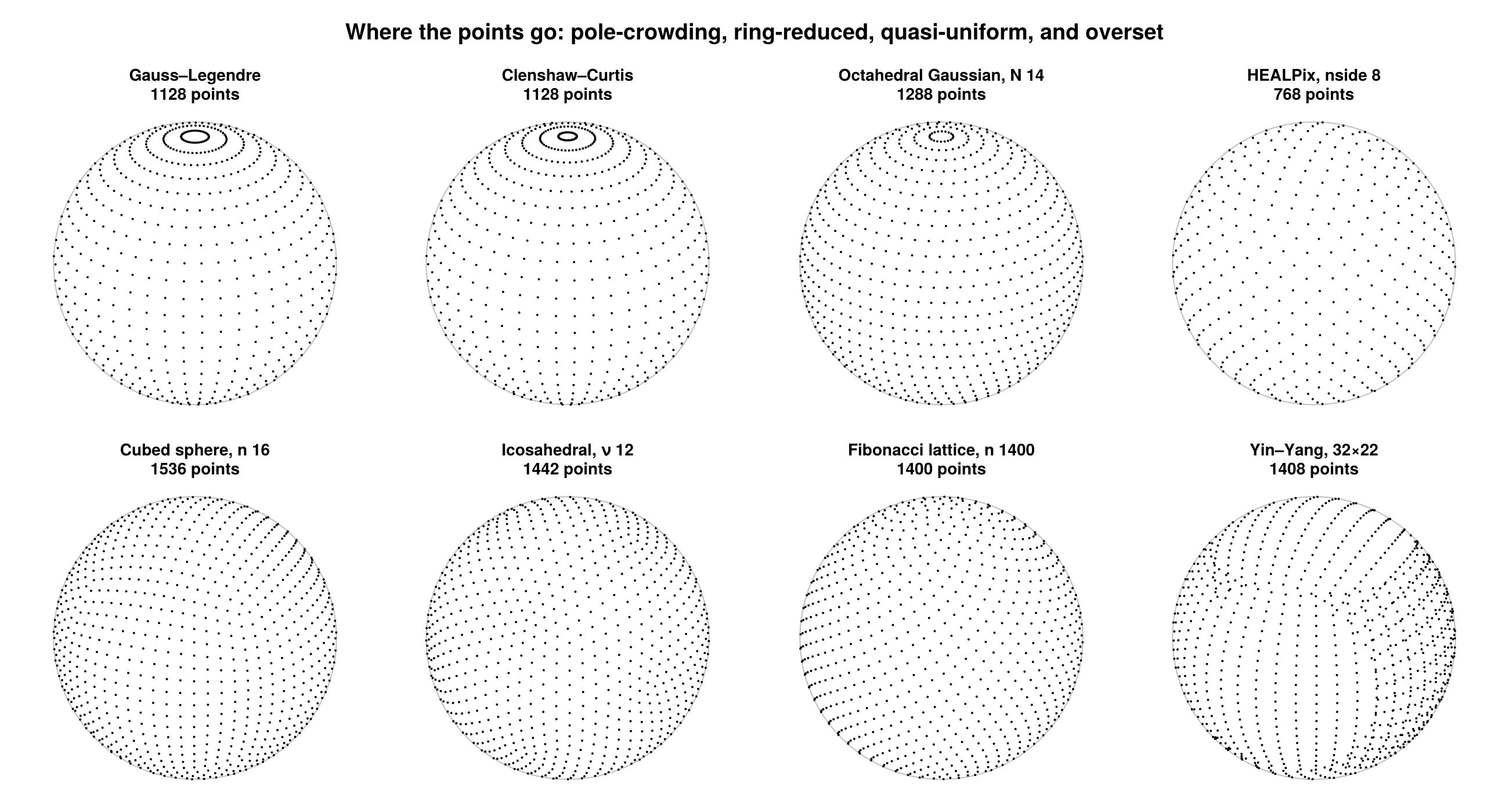
The central idea is that three questions people usually conflate are kept separate:
| question | answered by | examples |
|---|---|---|
| What is the metric? | Geometry | CartesianGeometry, SphericalGeometry |
| Where are the points? | SphericalSampling | Gauss–Legendre, HEALPix, cubed sphere, icosahedral, Yin–Yang |
| How is the data stored and connected? | Grids, Connectivity | structured, curvilinear, unstructured |
A Gauss–Legendre sampling can live in a structured grid under a spherical geometry; so can a lat–lon sampling. Changing one does not force a change in the others.
Installation
using Pkg
Pkg.add(url = "https://github.com/jbphyswx/FlowGeometries.jl")
Quick start
The package exports nothing. Import it qualified:
using FlowGeometries: FlowGeometries as FGA spherical grid from a spectral sampling:
geo  = FG.Geometry.SphericalGeometry()                                   # unit-agnostic; default Earth radius
grid = FG.Connectivity.structured_grid(FG.SphericalSampling.GaussLegendreSampling(), 64)       # 127 × 64 lon/lat

FG.Grids.coords(grid, 3, 5)          # (λ = …, φ = …) — named for the geometry, not (x, y)
FG.Grids.measure(grid, 3, 5)         # that cell's area
sum(FG.Grids.measure(grid)) / (4π * geo.R^2) # ≈ 1: the cells tile the sphere1.0000076786239283Nodes and quadrature weights together, from a single solve:
q = FG.SphericalSampling.spherical_quadrature(FG.SphericalSampling.GaussLegendreSampling(), 1024)
q.λ, q.φ, q.w                  # longitudes, latitudes, latitude weights
sum(q.w) # 2, i.e. ∫₋₁¹ dμ1.9999999999999998An unstructured grid on a quasi-uniform sampling, with exact dual-cell areas:
g = FG.Connectivity.unstructured_grid(FG.SphericalSampling.IcosahedralSampling(16))   # 2562 nodes
sum(FG.Grids.measure(g)) / (4π * FG.Geometry.SphericalGeometry().R^2) # 1.0 to machine precision
FG.Grids.neighbors(g, 1)                                     # this node's neighbours
FlowGeometries.Connectivity.MeshNeighbors{FlowGeometries.Grids.UnstructuredGrid{Float64, FlowGeometries.Geometry.SphericalGeometry{Float64}, 2, Tuple{Vector{Float64}, Vector{Float64}}, Vector{Float64}, FlowGeometries.Grids.AllActive{1}, Tuple{FlowGeometries.Grids.Periodic, FlowGeometries.Grids.Bounded}, Vector{Int32}, Vector{Int32}, Nothing}}(UnstructuredGrid{Float64}(2562), 1, true)Neighbours on a structured grid, without materializing anything:
out = Vector{Int}(undef, 8)
n = FG.Connectivity.neighbors!(out, grid, 3, 5; stencil = FG.Stencils.Moore(1)) # writes n indices8Conventions
- Nothing is exported, and nothing is rebound at the top level. Every name is reached through the submodule that defines it:
FG.Axes,FG.Geometry,FG.Stencils,FG.Discretization,FG.SphericalSampling,FG.Grids,FG.Connectivity,FG.Execution. - Coordinates are named by the geometry. A spherical grid has
grid.λ,grid.φ; a Cartesian one hasgrid.x,grid.y. Asking for the wrong one is an error, never a silent alias for the other. - Spherical coordinates are the polar frame
(λ, φ, r)— longitude, geographic latitude, radius — not east/north. - Cells are cell-centred. A sampling's points are cell centres, and the connectivity treats each point as one cell. The two never disagree.
f!means it writes into your buffers and allocates nothing beyond its return value — asserted in the test suite for every such form, at more than one problem size.- Nonstandard element types work.
Float32andBigFloatare supported throughout; algorithms that cannot reach a given precision defer to ones that can.