Spherical Sampling
A sampling answers: where are the points? It is independent of the metric and of how the data is stored.
The families
| sampling | layout | points | notes |
|---|---|---|---|
GaussLegendreSampling | tensor product | (2N−1) × N | exact quadrature to lmax = N−1 |
DriscollHealySampling | tensor product | 2N × N | equiangular, includes the north pole |
DriscollHealyEqualSampling | tensor product | N × N | the square DH1 layout |
ClenshawCurtisSampling | tensor product | (2N−1) × N | open — no polar points |
McEwenWiauxSampling | tensor product | (2L−1) × L | ~half the samples of classical DH |
LatLonSampling | tensor product | arbitrary | regional or global; no spectral claim |
HEALPixSampling | iso-latitude rings | 12·nside² | equal area by construction |
CubedSphereSampling | 6 panels | 6n² | quasi-uniform |
IcosahedralSampling | geodesic | 10ν²+2 | quasi-uniform; hexagonal dual |
YinYangSampling | 2 overlapping panels | 2·nlon·nlat | no polar singularity |
ScatteredSphericalSampling | arbitrary | any | for NUFFT-style paths |
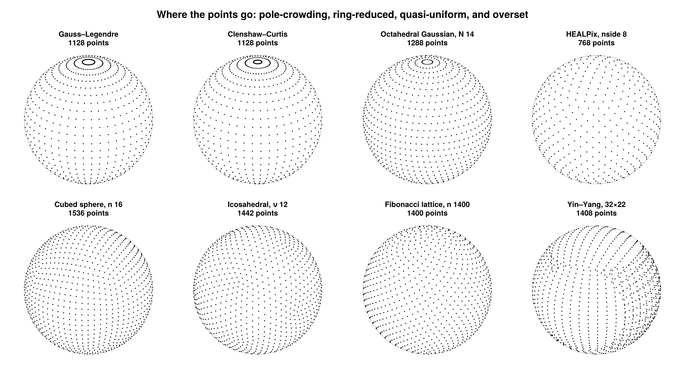
Gauss–Legendre and Clenshaw–Curtis put their points on iso-latitude rings that crowd toward the poles; HEALPix, the cubed sphere and the icosahedral geodesic are quasi-uniform. Yin–Yang is two overlapping panels, neither of which reaches a pole.
Traits
Ask a sampling what it is, and do not test its type:
FG.SphericalSampling.is_tensor_product(s)                       # fits an (nlon × nlat) structured grid?
FG.SphericalSampling.is_iso_latitude(s)                          # points lie on rings of constant φ?
FG.SphericalSampling.is_equal_area(s)                            # every cell the same area?
FG.SphericalSampling.admits_exact_bandlimited_quadrature(s) # weights integrate products exactly at `bandlimit`?trueThat last one is strict. Spectral analysis forms products of two degree-lmax fields, so it needs exactness to degree 2·lmax:
| sampling | exact for a single Pₗ | bandlimit | needs | exact? |
|---|---|---|---|---|
| Gauss–Legendre | 2N−1 | N−1 | 2N−2 | yes |
| Driscoll–Healy | N−1 | N/2−1 | N−2 | yes |
| Clenshaw–Curtis | N−1 | N−1 | 2N−2 | no |
Clenshaw–Curtis's band limit describes what its grid can represent; its quadrature only supports analysis to about (N−1)/2. Use Gauss–Legendre when the analysis has to be exact.
Sizing
FG.SphericalSampling.bandlimit(s, nlat)              # lmax this grid resolves
FG.SphericalSampling.nlat_for_bandlimit(s, 15)       # the inverse
FG.SphericalSampling.nlon_for_nlat(s, nlat)          # the matching longitude count
FG.SphericalSampling.axes_lengths(s, nlat)           # (; nlon, nlat)
FG.SphericalSampling.npoints(s, nlat) # total points496Axes, points and weights
Tensor-product samplings give separable axes; the rest give point lists.
ax = FG.SphericalSampling.spherical_axes(FG.SphericalSampling.GaussLegendreSampling(), 64)      # (; λ, φ) — 127 and 64 long
w  = FG.SphericalSampling.latitude_weights(FG.SphericalSampling.GaussLegendreSampling(), 64)    # 64 weights, Σw = 2
64-element Vector{Float64}:
0.0017832807216964326
0.004147033260562467
0.006504457968978363
0.008846759826363949
0.011168139460131126
0.013463047896718644
0.01572603047602472
0.01795171577569734
0.020134823153530212
0.02227017380838325
⋮
0.020134823153530212
0.01795171577569734
0.01572603047602472
0.013463047896718644
0.011168139460131126
0.008846759826363949
0.006504457968978363
0.004147033260562467
0.0017832807216964326If you need both, ask for both. Gauss–Legendre nodes and weights come out of one root solve; requesting them separately solves twice:
q = FG.SphericalSampling.spherical_quadrature(FG.SphericalSampling.GaussLegendreSampling(), 64) # (; λ, φ, w) — one solve(λ = [0.0, 0.049473900056532176, 0.09894780011306435, 0.14842170016959652, 0.1978956002261287, 0.2473695002826609, 0.29684340033919304, 0.3463173003957252, 0.3957912004522574, 0.4452651005087896 … 5.788446306614264, 5.8379202066707965, 5.887394106727329, 5.936868006783861, 5.986341906840393, 6.035815806896926, 6.085289706953458, 6.13476360700999, 6.184237507066522, 6.233711407123054], φ = [-1.5335125830545813, -1.4852145779583523, -1.4366313478480872, -1.3879836743385505, -1.3393115571950114, -1.2906276131055214, -1.241937060919817, -1.1932424462905298, -1.144545157917862, -1.0958460174998903 … 1.0958460174998903, 1.144545157917862, 1.1932424462905298, 1.241937060919817, 1.2906276131055214, 1.3393115571950114, 1.3879836743385505, 1.4366313478480872, 1.4852145779583523, 1.5335125830545813], w = [0.0017832807216964326, 0.004147033260562467, 0.006504457968978363, 0.008846759826363949, 0.011168139460131126, 0.013463047896718644, 0.01572603047602472, 0.01795171577569734, 0.020134823153530212, 0.02227017380838325 … 0.02227017380838325, 0.020134823153530212, 0.01795171577569734, 0.01572603047602472, 0.013463047896718644, 0.011168139460131126, 0.008846759826363949, 0.006504457968978363, 0.004147033260562467, 0.0017832807216964326])Every one of these has an in-place form that writes into your buffers and allocates nothing beyond its return value: spherical_axes!, latitude_weights!, spherical_quadrature!, spherical_points!.
λ = Vector{Float64}(undef, 127); φ = Vector{Float64}(undef, 64); w = similar(φ)
FG.SphericalSampling.spherical_quadrature!(λ, φ, w, FG.SphericalSampling.GaussLegendreSampling(), 64)
sum(w)1.9999999999999998Weights are normalized so Σw = ∫₀^π sinθ dθ = 2 for every sampling that has them. McEwen–Wiaux has none: its quadrature is built on an extension of the sphere to a torus, and the sine-series rule at its nodes is not exact even at l = 0, so asking for them raises.
Sampling-specific constructors
FG.SphericalSampling.cubed_sphere_points(n).panel |> unique     # 6n² cell centres + panel ids
length(FG.SphericalSampling.icosahedral_mesh(ν).triangles)      # 20ν² triangles
length(FG.SphericalSampling.icosahedral_vertices(ν).λ)          # 10ν²+2 points, no topology built
size(FG.SphericalSampling.yin_yang_panels(nlon, nlat).yang.λ)
FG.SphericalSampling.healpix_npix(nside), FG.SphericalSampling.healpix_nring(nside)
(768, 31)yin_yang_panels returns two different shapes. The yin panel is a separable lat–lon patch in its own frame, so it is a pair of axes; yang is that panel rotated onto the sphere, separable in neither global longitude nor latitude, so it is a pair of nlon × nlat fields.
icosahedral_vertices! writes the points straight into your buffers with no mesh built at all, so its allocation count does not grow with ν.
Ring grids and quasi-uniform lattices
A reduced Gaussian grid keeps the Gaussian latitudes but gives each ring only as many longitudes as its circumference warrants, so it is not a tensor product:
oct = FG.SphericalSampling.OctahedralGaussianSampling(80)     # ECMWF octahedral, N = 80
FG.SphericalSampling.nrings(oct), FG.SphericalSampling.npoints(oct), 4 * 80 * (80 + 9)
(160, 28480, 28480)first(FG.SphericalSampling.nlon_per_ring(oct), 4) # 20 at the pole, +4 per ring4-element Vector{Int64}:
20
24
28
32Its latitude weights are Gauss–Legendre's, so the quadrature is exact; the longitude factor varies by ring because the ring populations do:
w = FG.SphericalSampling.latitude_weights(oct)
counts = FG.SphericalSampling.nlon_per_ring(oct)
sum(w), sum(w[j] * (2π / counts[j]) * counts[j] for j in eachindex(counts)) / 4π
(1.9999999999999998, 1.0000000000000004)Walking a map ring by ring
nlon_per_ring builds the whole table. To take rings one at a time, nlon_in_ring and ring_range answer for a single ring in O(1) and allocate nothing, so a per-ring transform or a zonal reduction carries no running offset and no table:
SS = FG.SphericalSampling
pts = SS.spherical_points(oct)
zonal = [sum(view(pts.φ, SS.ring_range(oct, r))) / SS.nlon_in_ring(oct, r)
         for r in 1:SS.nrings(oct)]
zonal[1], zonal[end]                  # each ring is at one latitude, so this is that latitude
(1.555813014222234, -1.555813014222234)Both are defined for every sampling laid out in rings — the octahedral and tabulated reduced Gaussians, HEALPix, and the tensor-product grids, which take their nlat first:
SS.ring_range(SS.HEALPixSampling(4), 3), SS.ring_range(SS.GaussLegendreSampling(), 8, 3)(13:24, 31:45)The Fibonacci lattice spreads points one per equal-area band with a golden-angle longitude step, which gives a quasi-uniform set with no polar clustering and no panel seams:
fib = FG.SphericalSampling.spherical_points(FG.SphericalSampling.FibonacciSampling(1000))
extrema(diff(sin.(fib.φ)))            # exactly equal steps in z
(0.0019999999999997797, 0.002000000000000113)HEALPix pixel indexing
SS = FG.SphericalSampling
θ, ϕ = SS.pix2ang(8, 100)             # RING by default
SS.ang2pix(8, θ, ϕ)100SS.ring2nest(8, 100), SS.nest2ring(8, SS.ring2nest(8, 100))(167, 100)Nested() selects the quadtree ordering, which needs nside to be a power of two; Ring() works for any nside. pix2vec/vec2pix are the same maps through a unit vector.
ring_info describes a whole iso-latitude ring at once, so a map can be walked ring by ring without decoding every pixel. Ring widths run 4, 8, … through the polar cap, hold at 4·nside across the equatorial belt, then shrink symmetrically:
[SS.ring_info(4, r).ringpix for r in 1:(4 * 4 - 1)]15-element Vector{Int64}:
4
8
12
16
16
16
16
16
16
16
16
16
12
8
4info = SS.ring_info(4, 6)
info.startpix, info.ringpix, info.latitude, info.shifted(56, 16, 0.3398369094541218, true)The rings tile the map exactly — startpix is contiguous and the widths sum to 12·nside²:
rings = [SS.ring_info(4, r) for r in 1:15]
sum(i -> i.ringpix, rings) == 12 * 4^2, rings[1].startpix == 0
(true, true)Points sit at cell centres
Every sampling here places points at cell centres. Sampling the panel edges makes adjacent panels emit coincident points while the connectivity folds those same edges onto a different panel; points and topology then disagree, and a grid built from them carries duplicate nodes and zero-area cells. Cell centres also give the degenerate sizes (n = 1, nlon = 1) from the same formula, with no special case.