Grids
A grid answers: how is the data stored? It pairs a geometry with coordinates, a per-cell measure and an activity mask.
| type | coordinates | use |
|---|---|---|
StructuredGrid | one 1-D axis per direction | rectilinear: lat–lon, any tensor-product sampling |
CurvilinearGrid | one N-D array per direction | logically rectangular, geometrically warped |
HEALPixGrid | none — (nside, pixel) arithmetic | the HEALPix pixelization |
CubedSphereGrid | none — (n, cell) arithmetic | the gnomonic cubed sphere |
YinYangGrid | none — (nlon, nlat, cell) arithmetic | Kageyama–Sato overset panels |
IcosahedralGrid | none — (ν, id) arithmetic | geodesic, 12 pentagons |
RingGrid | one value per ring | reduced Gaussian, octahedral |
UnstructuredGrid | one value per node, plus CSR neighbours | scattered points, an arbitrary mesh |
The first two store coordinates because a warped mesh's are arbitrary; the last stores them because a node set's are the caller's. The five in between store none, or O(√n): a cell's position, its neighbours and its area are closed-form in the layout's parameters, so they hold those parameters instead. HEALPixGrid is the same size at nside = 1024 — 12.6 million pixels — as at nside = 1. Ask for the dense cloud with Grids.materialize when something outside needs it.
Building one
using FlowGeometries: FlowGeometries as FG

# From a sampling — the usual route
grid = FG.Connectivity.structured_grid(FG.SphericalSampling.ClenshawCurtisSampling(), 64)
g    = FG.Grids.HEALPixGrid(16)
rg   = FG.Grids.RingGrid(FG.SphericalSampling.OctahedralGaussianSampling(64))
cs   = FG.Grids.CubedSphereGrid(24)
yy   = FG.Grids.YinYangGrid(32, 22)
ico  = FG.Grids.IcosahedralGrid(16)

# Or directly, in any number of dimensions; the mask is optional
sg  = FG.Grids.StructuredGrid(FG.Geometry.SphericalGeometry(), λaxis, φaxis, mask)
cg  = FG.Grids.CurvilinearGrid(FG.Geometry.SphericalGeometry(), λ2d, φ2d, mask)
g4  = FG.Grids.StructuredGrid(FG.Geometry.CartesianGeometry(),
                              0:1.0:3, 0:1.0:3, 0:1.0:3, 0:1.0:3)  # 4-D, all active
size(g4)
(4, 4, 4, 4)A formula layout's storage does not depend on its resolution, and the arithmetic is what answers every per-cell question:
g1024 = FG.Grids.HEALPixGrid(1024)                 # 12 582 912 pixels
Base.summarysize(g) == Base.summarysize(g1024), length(g1024)
(true, 12582912)FG.Grids.coords(g, 100), FG.Grids.measure(g, 100), collect(FG.Grids.neighbors(g, 100))((λ = 3.478191866474414, φ = 1.2116520114493072), 1.6603661194980087e11, [51, 73, 74, 99, 101, 130, 131, 165])λ, φ = FG.Grids.materialize(g) # the dense cloud, asked for explicitly
length(λ)3072# The panel layouts answer the same way, and `sum(measure)` is the region they tile
sum(FG.Grids.measure(cs)) / (4π * FG.Geometry.radius(FG.Grids.grid_geometry(cs))^2),
sum(FG.Grids.measure(yy)) / (4π * FG.Geometry.radius(FG.Grids.grid_geometry(yy))^2)(1.0, 1.0606601717798212)The common interface
Everything below works on every architecture:
out = zeros(2)
FG.Grids.coords(grid, i, j)                        # (λ = …, φ = …) or (x = …, y = …)
FG.Grids.coords!(out, grid, i, j)                  # into your buffer
FG.Grids.coords(NTuple{2,Float64}, grid, i, j)     # a specific storage type
FG.Grids.measure(grid, i, j)                       # cell area / volume / control-volume size
FG.Grids.isactive(grid, i, j)                      # participates in the domain?
collect(FG.Grids.neighbors(grid, i, j))            # lazy iterator over neighbour indices
size(grid), length(grid), FG.Grids.size_tuple(grid)
FG.Grids.isperiodic(grid, 1), FG.Grids.period(grid, 1)
(true, 6.283185307179586)Coordinates are also reachable by their geometry-correct names — grid.λ, grid.φ on a sphere; grid.x, grid.y on a plane.
Cell measure is stored factored
On a rectilinear grid every measure this package supports is a product of one factor per axis: Cartesian Δx·Δy·Δz, spherical R²cosφ·Δλ·Δφ = (Δλ)·(R²cosφ·Δφ). A StructuredGrid stores those ∑ Nᵈ factors, and the ∏ Nᵈ products come out of them.
m = FG.Grids.measure(grid)           # a SeparableMeasure — a real AbstractArray
m[3, 5]                        # indexes exactly like the dense outer product
sum(m)                         # ∏ᵈ ∑ᵢ wᵈᵢ — O(∑ Nᵈ) against the dense O(∏ Nᵈ)
FG.Grids.measure_factors(grid)       # the per-axis factors, or `nothing`
FG.Grids.measure_array(grid)         # materialize densely, if you really need it
127×64 Matrix{Float64}:
2.41912e9 7.25153e9 1.20665e10 … 1.20665e10 7.25153e9 2.41912e9
2.41912e9 7.25153e9 1.20665e10 1.20665e10 7.25153e9 2.41912e9
2.41912e9 7.25153e9 1.20665e10 1.20665e10 7.25153e9 2.41912e9
2.41912e9 7.25153e9 1.20665e10 1.20665e10 7.25153e9 2.41912e9
2.41912e9 7.25153e9 1.20665e10 1.20665e10 7.25153e9 2.41912e9
2.41912e9 7.25153e9 1.20665e10 … 1.20665e10 7.25153e9 2.41912e9
2.41912e9 7.25153e9 1.20665e10 1.20665e10 7.25153e9 2.41912e9
2.41912e9 7.25153e9 1.20665e10 1.20665e10 7.25153e9 2.41912e9
2.41912e9 7.25153e9 1.20665e10 1.20665e10 7.25153e9 2.41912e9
2.41912e9 7.25153e9 1.20665e10 1.20665e10 7.25153e9 2.41912e9
⋮ ⋱
2.41912e9 7.25153e9 1.20665e10 1.20665e10 7.25153e9 2.41912e9
2.41912e9 7.25153e9 1.20665e10 1.20665e10 7.25153e9 2.41912e9
2.41912e9 7.25153e9 1.20665e10 … 1.20665e10 7.25153e9 2.41912e9
2.41912e9 7.25153e9 1.20665e10 1.20665e10 7.25153e9 2.41912e9
2.41912e9 7.25153e9 1.20665e10 1.20665e10 7.25153e9 2.41912e9
2.41912e9 7.25153e9 1.20665e10 1.20665e10 7.25153e9 2.41912e9
2.41912e9 7.25153e9 1.20665e10 1.20665e10 7.25153e9 2.41912e9
2.41912e9 7.25153e9 1.20665e10 … 1.20665e10 7.25153e9 2.41912e9
2.41912e9 7.25153e9 1.20665e10 1.20665e10 7.25153e9 2.41912e9Indexing, broadcasting and collect behave exactly as for the dense array, and the values are bit-identical. At 2000² the measure is 0.046 MiB against 61.0 MiB dense, and faster to read on every access pattern measured: the factors stay in cache while a 61 MiB array is DRAM-bound. See Performance.
Operations that keep the measure a product stay factored, so a unit conversion does not undo the saving: scaling, a multiplicative map (abs, abs2, sqrt, inv), and a factor-wise product or quotient of two measures.
km² = m ./ 1e6
typeof(km²).name.name, Base.summarysize(km²), sum(km²) ≈ sum(m) / 1e6
(:SeparableMeasure, 1624, true)Anything else materializes, correct and dense. exp is the clean example: it is not multiplicative, so exp(∏wᵈ) ≠ ∏exp(wᵈ) and there is no factored form to keep. A negative scale materializes too, non-negative factors being an invariant the findmax/findmin shortcut relies on.
typeof(exp.(m)).name.name, typeof((-1.0) .* m).name.name(:Array, :Array)sum being O(∑Nᵈ) is also what stops show from adding eight million numbers to print one line.
Masks
FG.Grids.mask(grid)                  # the mask array
FG.Grids.isactive(grid, i, j) # false = excluded (land, say)trueWhen every cell participates the mask is AllActive, which stores its size and nothing else — getindex folds to a constant and count is length without a scan. Pass a real BitArray or Array{Bool} when you need to exclude cells.
Curvilinear corners
CurvilinearGrid's exact quadrilateral cell area comes from its cell vertices — the spherical excess of the two triangles through the four corner directions on a sphere, the shoelace area on a plane.
cg2 = FG.Grids.CurvilinearGrid(geo, λ2d, φ2d, mask; x_corner = λc, y_corner = φc)
size(FG.Grids.corners(cg2, 1)), FG.Grids.corner_coords(cg2, i, j)
((64, 33), (λ = 0.14959965017094254, φ = 1.1780972450961724))Supply x_corner/y_corner when your source model ships its own cell-vertex grid; otherwise they are reconstructed from the centres, which needs at least a 2×2 grid.
Vertices you supply are kept on the grid. Reconstructed ones are input to the area kernel, and are kept only if you ask — one array per direction, one larger in every direction:
lean = FG.Grids.CurvilinearGrid(geo, λ2d, φ2d, mask)
full = FG.Grids.CurvilinearGrid(geo, λ2d, φ2d, mask; keep_corners = true)
FG.Grids.has_corners(lean), FG.Grids.has_corners(full),
    FG.Grids.measure(lean) == FG.Grids.measure(full),
    round(Base.summarysize(lean) / Base.summarysize(full); digits = 2)
(false, true, true, 0.59)A curvilinear grid takes any number of directions — one N-D array each, mask last. Beyond 2-D the cell measure is yours to pass: the corner-area kernel is an exact-quadrilateral algorithm with no N-D generalization here, so asking it for a 3-D measure raises.
cart = FG.Geometry.CartesianGeometry()
X = [x for x in 0.0:1.0:3.0, _ in 1:3, _ in 1:2]
Y = [y for _ in 1:4, y in 0.0:2.0:4.0, _ in 1:2]
Z = [z for _ in 1:4, _ in 1:3, z in 0.0:0.5:0.5]
cg3 = FG.Grids.CurvilinearGrid(cart, X, Y, Z, fill(1.0, 4, 3, 2), trues(4, 3, 2))
size(cg3), FG.Grids.coordinate_names(cg3), FG.Grids.coords(cg3, 2, 3, 2)
((4, 3, 2), (:x, :y, :z), (x = 1.0, y = 4.0, z = 0.5))The measure goes either before the mask, as above, or as the measure keyword — the same array either way:
FG.Grids.measure(FG.Grids.CurvilinearGrid(cart, X, Y, Z, trues(4, 3, 2);
                                          measure = fill(1.0, 4, 3, 2))) ==
FG.Grids.measure(cg3)trueNode grids generalize the same way, with the coordinates as a tuple — a run of vectors cannot say how many of them are coordinates, where a curvilinear grid counts them from ndims(mask):
nodes = FG.Grids.UnstructuredGrid(cart, (rand(6), rand(6), rand(6)), ones(6), trues(6))
FG.Grids.coordinate_names(nodes), FG.Grids.coords(nodes, 4)
((:x, :y, :z), (x = 0.2369327207598021, y = 0.6981699943233624, z = 0.8182045639473753))Cell areas on the spherical node sets
Cell areas are an exact closed form, dispatched on the sampling — never a uniform 4πR²/N fallback, which is right only for equal-area samplings and silently wrong elsewhere (icosahedral dual cells span a min/max ratio of 0.52).
| layout / sampling | cell areas |
|---|---|
HEALPixGrid | uniform 4πR²/N — exact by construction, and stored as one number |
CubedSphereGrid | exact solid angle of the cell's own gnomonic rectangle |
YinYangGrid | lat–lon patch area, R²Δλ·2sin(Δφ/2)·cosφ |
RingGrid | R²·(2π/nlonᵣ)·wᵣ from the ring's Gaussian weight |
IcosahedralGrid | the spherical Voronoi dual, from the vertex's own incident triangles |
| arbitrary points | Voronoi areas, via the Quickhull or DelaunayTriangulation extension |
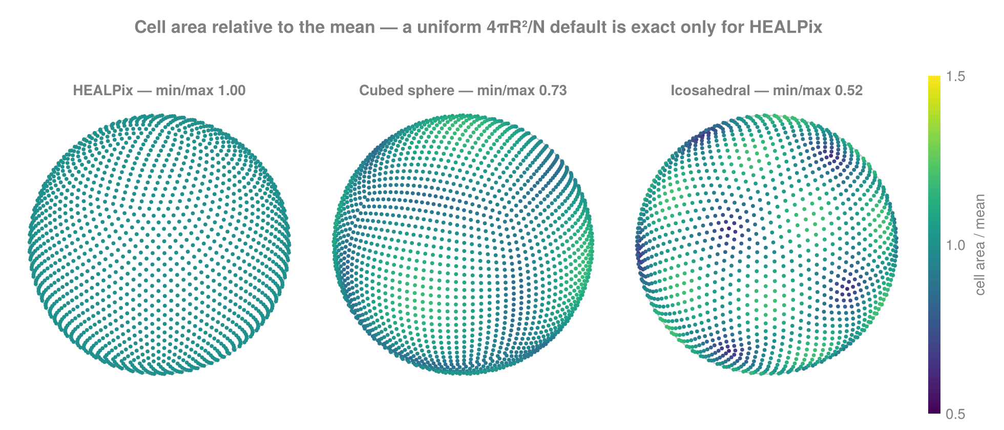
Only HEALPix is one flat colour. The dark spots on the icosahedral panel are its twelve pentagons — the smallest cells on the mesh, and the reason a uniform default is off by nearly a factor of two between the largest and smallest cell there.
Every closed form here sums to 4πR² to machine precision — with the documented Yin–Yang excess — and needs no optional dependency. On the node sets, pass areas = … to supply your own.
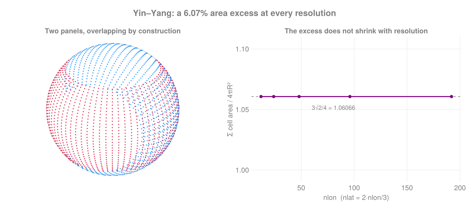
The two panels overlap by construction, so their cell areas sum to 3√2πR² — 6.07% more than the sphere, at every resolution. The excess is the overlap itself, and it does not shrink with the mesh. Integrating over both panels needs a partition-of-unity weight for the shared region, which is a modelling choice made on top of these areas.